Little by Little: Optimisation with analysis and gradients
Problems for with a known objective function or observable gradient is known can be solved efficiently through analysis or gradient descent/ascent.
This article will formalise the concept of optimisation and introduce optimisation with analysis and gradient descent.
This is the second part of a series on optimisation. Head to the first part to develop an intuition of optimisation problems with very little maths involved.
As mentioned in the first part, an optimisation problem refers to minimising or maximising an objective function, depending on a set of decision variables, with respect to a list of constraints.
Example: A private company producing tables and chairs would try to maximise its profit (revenue minus costs, the objective function) depending on the quantities it produces (decision variables). Some constraints could involve the current capital or number of workers the firm hires.
Formalising this, an optimisation problem is:
\[ \begin{align*} \min_{\mathbf{x} \in S} \quad & f(\mathbf{x}) \end{align*} \]
or
\[ \begin{align*} \max_{\mathbf{x} \in S} \quad & f(\mathbf{x}) \end{align*} \]
where \(S\) is the search space, \(\mathbf{x}\) a vector of decision variables, and \(f\) is the objective function.
The optimisation methods at our disposal depend on the amount of information we have about a problem.
Using analysis
In the production example, if we are given both the revenue and cost functions, it may be possible to find the solution to the problem. To simplify, let’s only consider \(q\) the quantity of tables to produce.
Let’s define:
- Cost function: \(C(q) = 2q^2 + 200q + 100\)
- Revenue function: \(R(q) = p q\)
Deriving the profits from revenues minus costs:
\[ \Pi(q) = R(q) - C(q) = p q - \left(2 q^2 + 200 q + 100\right) \]
Simplifying:
\[ \Pi(q) = p q - 2 q^2 - 200 q - 100 = (p - 200) q - 2 q^2 - 100 \]
We can then use first and second derivatives to find the critical points of this function, and determine whether they are maximums or minimums.
\[ \frac{d\Pi}{dq} = (p - 200) - 4 q \]
The expression \(\frac{d\Pi}{dq}\) represents the derivative of profits with respects to \(q\) the quantity of tables produced. In English, this represents the change in the profit function (\(\Pi\)) generated by a very small increase in \(q\).
Setting the first derivative to 0 allows us to find the critical point of the function (reached at \(q^*\))
\[ (p - 200) - 4 q = 0 \implies 4 q = p - 200 \implies q^* = \frac{p - 200}{4} \]
However, a critical point could be either a minimum or maximum. To make sure that this is a maximum, we need to check if the function is concave at this critical point. We can do that by ensuring that the second derivative at this point is negative.
Checking the sign of the second derivative:
\[ \frac{d^2\Pi}{dq^2} = -4 \]
Since \(-4 < 0\), the second derivative is negative, confirming that \(q^*\) is a maximum.
Suppose the price per table is €400:
\[ q^* = \frac{400 - 200}{4} = \frac{200}{4} = 50 \]
Thus, the company maximises profit by producing 50 tables.
This process is highly efficient as only a few calculations are needed to get to the result. This would take less than a millisecond on a personal computer.
Observing the gradient
Other than analysis, we can use gradient descent to solve more complex problems. Let’s consider the following functions:
Revenue function:
\[ R(q_t, q_c) = p_t q_t + p_c q_c \]
Cost functions:
For tables:
\[ C_1(q_t) = 2 q_t^2 + 200 q_t + 100 \]
For chairs:
\[ C_2(q_c) = 3 q_c^2 + 150 q_c + 80 \]
Total cost:
\[ C(q_t, q_c) = C_1(q_t) + C_2(q_c) \]
Profit function:
\[ \Pi(q_t, q_c) = R(q_t, q_c) - C(q_t, q_c) \]
Let’s specify:
- Price per table: \(p_t = 400\)
- Price per chair: \(p_c = 250\)
Therefore, the profit function is:
\[ \begin{align*} \Pi(q_t, q_c) &= 400 q_t + 250 q_c - \left(2 q_t^2 + 200 q_t + 100 + 3 q_c^2 + 150 q_c + 80\right) \\ &= 400 q_t + 250 q_c - 2 q_t^2 - 200 q_t - 100 - 3 q_c^2 - 150 q_c - 80 \\ &= (200 q_t - 2 q_t^2) + (100 q_c - 3 q_c^2) - 180 \end{align*} \]
Simplifying:
\[ \Pi(q_t, q_c) = 200 q_t - 2 q_t^2 + 100 q_c - 3 q_c^2 - 180 \]
Finding the maximum analytically is already more challenging than the univariate case, though definitely doable. We will solve this using gradient descent to illustrate this different approach.
The gradient of a function (noted \(\nabla f\)) is the vector of partial derivatives. One of its properties is that it always points to the direction of steepest ascent of the function.
As an example, the gradient of the function \(f(x,y)=x^2 + y^2\) is:
\[ \nabla f(x, y) = \begin{pmatrix} \dfrac{\partial f}{\partial x} \\[8pt] \dfrac{\partial f}{\partial y} \end{pmatrix} = \begin{pmatrix} 2x \\[8pt] 2y \end{pmatrix} \]
Following the opposite direction of this gradient will lead to the steepest decrease in the function. In practice, following the opposite of the gradient would mean updating \(x\) and \(y\) by subtracting a fraction of the gradient. This fraction is called the learning rate (noted \(\alpha\)). More on the learning rate below.
\[ \begin{pmatrix} x_{t+1} \\[8pt] y_{t+1} \end{pmatrix} = \begin{pmatrix} x_t \\[8pt] y_t \end{pmatrix} - \alpha \cdot \nabla f(x_t, y_t) \]
Trying to find a minimum to the function starting from the random guess \(x_0=3\) and \(y_0=2\), using \(0.1\) as learning rate, we get:
\[ \begin{pmatrix} x_{1} \\ y_{1} \end{pmatrix} = \begin{pmatrix} 3 \\ 2 \end{pmatrix} - 0.1 \cdot \begin{pmatrix} 6 \\ 4 \end{pmatrix} = \begin{pmatrix} 2.4 \\ 1.6 \end{pmatrix} \]
\[ \begin{pmatrix} x_{2} \\ y_{2} \end{pmatrix} = \begin{pmatrix} 2.4 \\ 1.6 \end{pmatrix} - 0.1 \cdot \begin{pmatrix} 4.8 \\ 3.2 \end{pmatrix} = \begin{pmatrix} 1.92 \\ 1.28 \end{pmatrix} \]
\[ \begin{pmatrix} x_{3} \\ y_{3} \end{pmatrix} = \begin{pmatrix} 1.92 \\ 1.28 \end{pmatrix} - 0.1 \cdot \begin{pmatrix} 3.84 \\ 2.56 \end{pmatrix} = \begin{pmatrix} 1.536 \\ 1.024 \end{pmatrix} \]
\[ \vdots \]
This process will slowly converge to \(x_n = 0\) and \(y_n = 0\).
\[ \lim_{n \to \infty} \begin{pmatrix} x_n \\ y_n \end{pmatrix} = \begin{pmatrix} 0 \\ 0 \end{pmatrix} \]
Similarly, following its direction will lead to the steepest increase in the function. \[ \begin{pmatrix} x_{t+1} \\ y_{t+1} \end{pmatrix} = \begin{pmatrix} x_t \\ y_t \end{pmatrix} + \alpha \cdot \nabla f(x_t,y_t) \]
Going back to tables and chairs, the gradient vector of the profit function:
\[ \Pi(q_t, q_c) = 200 q_t - 2 q_t^2 + 100 q_c - 3 q_c^2 - 180 \]
It is the vector of its partial derivatives:
\[ \nabla \Pi(q_t, q_c) = \begin{pmatrix} \dfrac{\partial \Pi}{\partial q_t} \\[8pt] \dfrac{\partial \Pi}{\partial q_c} \end{pmatrix} \]
Partial derivative with respect to \(q_t\):
\[ \frac{\partial \Pi}{\partial q_t} = 200 - 4 q_t \]
Partial derivative with respect to \(q_c\):
\[ \frac{\partial \Pi}{\partial q_c} = 100 - 6 q_c \]
The gradient of \(\Pi\) is therefore: \[ \nabla \Pi(q_t, q_c) = \begin{pmatrix} 200 - 4q_t \\ 100 - 6q_c \end{pmatrix} \]
Starting from the following guess with \(\alpha = 0.5\):
- \(q_t^{(0)} = 10\)
- \(q_c^{(0)} = 10\)
and applying the gradient ascent update rule, we get:
\[ \begin{aligned} \begin{pmatrix} q_t^{(1)} \\ q_c^{(1)} \end{pmatrix} &= \begin{pmatrix} 10 \\ 10 \end{pmatrix} + 0.05 \cdot \begin{pmatrix} 200 - 4q_t^{(0)} \\ 100 - 6q_c^{(0)} \end{pmatrix} \\ &= \begin{pmatrix} 10 \\ 10 \end{pmatrix} + 0.05 \cdot \begin{pmatrix} 200 - 40 \\ 100 - 60 \end{pmatrix} \\ &= \begin{pmatrix} 10 \\ 10 \end{pmatrix} + 0.05 \cdot \begin{pmatrix} 160 \\ 40 \end{pmatrix} \\ &= \begin{pmatrix} 10 \\ 10 \end{pmatrix} + \begin{pmatrix} 8 \\ 2 \end{pmatrix} \\ &= \begin{pmatrix} 18 \\ 12 \end{pmatrix} \end{aligned} \]
\[ \begin{aligned} \begin{pmatrix} q_t^{(2)} \\ q_c^{(2)} \end{pmatrix} &= \begin{pmatrix} 18 \\ 12 \end{pmatrix} + 0.05 \cdot \begin{pmatrix} 200 - 4q_t^{(1)} \\ 100 - 6q_c^{(1)} \end{pmatrix} \\ &= \begin{pmatrix} 18 \\ 12 \end{pmatrix} + 0.05 \cdot \begin{pmatrix} 200 - 72 \\ 100 - 72 \end{pmatrix} \\ &= \begin{pmatrix} 18 \\ 12 \end{pmatrix} + 0.05 \cdot \begin{pmatrix} 128 \\ 28 \end{pmatrix} \\ &= \begin{pmatrix} 18 \\ 12 \end{pmatrix} + \begin{pmatrix} 6.4 \\ 1.4 \end{pmatrix} \\ &= \begin{pmatrix} 24.4 \\ 13.4 \end{pmatrix} \end{aligned} \]
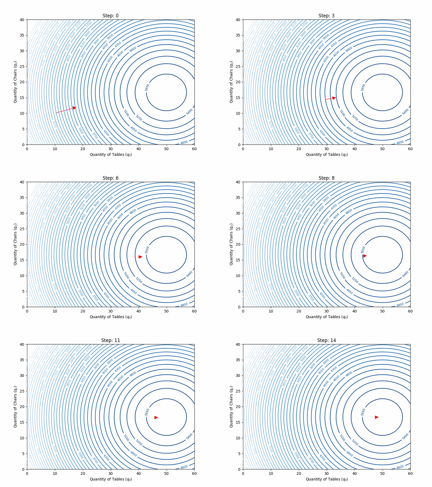
The full search is illustrated in the animation below:

Code to generate the animation
import numpy as np
import matplotlib.pyplot as plt
from matplotlib.animation import FuncAnimation
from matplotlib.patches import FancyArrowPatch

def profit(q1, q2):
    return 200 * q1 - 2 * q1**2 + 100 * q2 - 3 * q2**2 - 180

def grad_profit(q1, q2):
    dp_dq1 = 200 - 4 * q1
    dp_dq2 = 100 - 6 * q2
    return np.array([dp_dq1, dp_dq2])

# Gradient ascent parameters
alpha = 0.05
steps = 15
history = []

# Initial guess
q1 = 10
q2 = 10

for _ in range(steps):
    gradient = grad_profit(q1, q2)
    history.append((q1, q2, gradient))
    q1 += alpha * gradient[0]
    q2 += alpha * gradient[1]

# Prepare for the animation
fig, ax = plt.subplots(figsize=(8, 6))
q1_vals = np.linspace(0, 60, 200)
q2_vals = np.linspace(0, 40, 200)
Q1, Q2 = np.meshgrid(q1_vals, q2_vals)
Pi = profit(Q1, Q2)
contours = ax.contour(Q1, Q2, Pi, levels=50, cmap="Blues")
plt.clabel(contours, inline=True, fontsize=8)
ax.set_title('Profit as a Function of Tables and Chairs')
ax.set_xlabel('Quantity of Tables ($q_t$)')
ax.set_ylabel('Quantity of Chairs ($q_c$)')

prev_arrow = None

def init():
    ax.set_xlim(0, 60)
    ax.set_ylim(0, 40)
    return []

def update(frame):
    global prev_arrow
    q1, q2, gradient = history[frame]
    # Remove previous arrow
    if prev_arrow is not None:
        prev_arrow.remove()
    # Scale gradient for arrow visualization
    norm_gradient = gradient * alpha
    dq1, dq2 = norm_gradient
    # Draw an arrow showing the gradient ascent direction
    arrow = FancyArrowPatch(
      (q1, q2), (q1 + dq1, q2 + dq2),
      arrowstyle='-|>', color='r', mutation_scale=20
    )
    ax.add_patch(arrow)
    prev_arrow = arrow
    ax.set_title(f'Step: {frame}')
    return [arrow]

ani = FuncAnimation(fig, update, frames=range(len(history)), init_func=init, blit=True, interval=1000)
plt.show()
Do we even need a learning rate?
The gradient descent update rule is the following:
\[ f(\mathbf{x_{t+1}}) = f(\mathbf{x_t}) - \alpha \cdot \nabla f(\mathbf{x_t}) \]
With \(\mathbf{x}\) the vector of inputs of the function \(f\).
Why not add or subtract the gradient directly? Wouldn’t we reach the optimum faster?
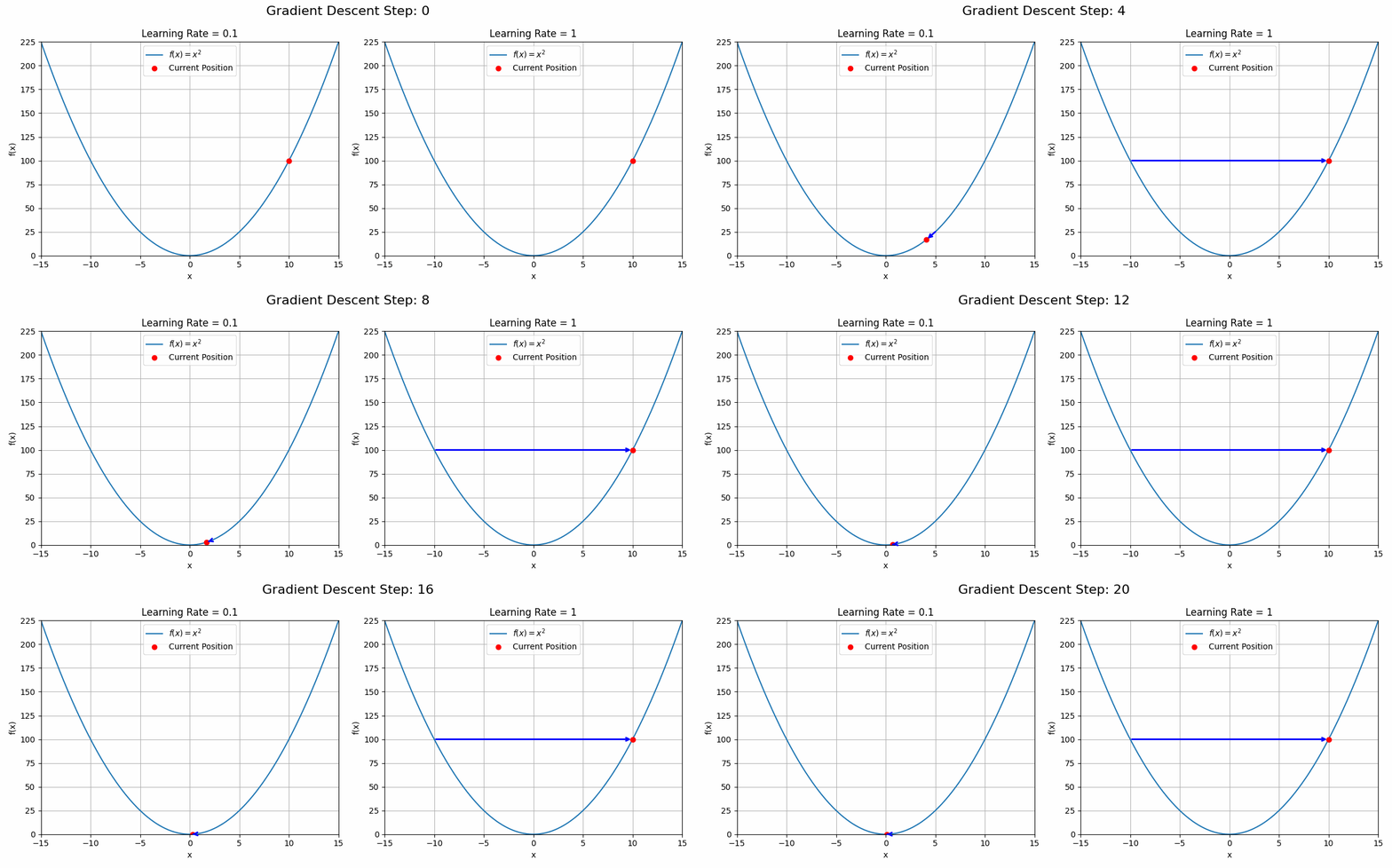
Because a picture is worth a thousand words (and a gif maybe more), the animation below shows what could happen with a learning rate set to 1 (equivalent to no learning rate at all).

Code to generate the animation
import numpy as np
import matplotlib.pyplot as plt
from matplotlib.animation import FuncAnimation

def gradient_descent(learning_rate, steps, x_initial):
    x = x_initial
    history = [x]
    for _ in range(steps):
        grad = 2 * x  # Gradient of f(x) = x^2 is f'(x) = 2x
        x = x - learning_rate * grad
        history.append(x)
    return history

x_initials = [10, 10]  # Starting points for each learning rate
steps = 20            # Number of steps
learning_rates = [0.1, 1]

# Prepare histories for both learning rates
histories = []
for lr, x_init in zip(learning_rates, x_initials):
    history = gradient_descent(lr, steps, x_init)
    histories.append(history)

# Prepare the plot
fig, axes = plt.subplots(1, 2, figsize=(12, 5))
x_vals = np.linspace(-15, 15, 400)
y_vals = x_vals ** 2

# Initialize plots
lines = []
arrows = []
for ax, lr in zip(axes, learning_rates):
    ax.plot(x_vals, y_vals, label='$f(x) = x^2$')
    line, = ax.plot([], [], 'ro', label='Current Position')
    lines.append(line)
    arrows.append(None)  # Placeholder for arrows
    ax.set_title(f'Learning Rate = {lr}')
    ax.set_xlabel('x')
    ax.set_ylabel('f(x)')
    ax.set_xlim(-15, 15)
    ax.set_ylim(0, 225)
    ax.legend()
    ax.grid(True)

def animate(i):
    fig.suptitle(f'Gradient Descent Step: {i}', fontsize=16)
    for idx, (line, history, ax) in enumerate(zip(lines, histories, axes)):
        if i < len(history):
            x_current = history[i]
        else:
            x_current = history[-1]
        y_current = x_current ** 2
        line.set_data([x_current], [y_current])

        # Remove previous arrow if exists
        if arrows[idx] is not None:
            arrows[idx].remove()

        # Draw arrow from previous point to current point
        if i > 0:
            x_prev = history[i - 1]
            y_prev = x_prev ** 2
            arrow = ax.annotate(
                '',
                xy=(x_current, y_current),
                xytext=(x_prev, y_prev),
                arrowprops=dict(arrowstyle='->', color='blue', lw=2),
            )
            arrows[idx] = arrow
        else:
            arrows[idx] = None  # No arrow in the first frame

    return lines + [arrow for arrow in arrows if arrow is not None]

ani = FuncAnimation(fig, animate, frames=steps + 1, interval=500, blit=True)
plt.tight_layout()
plt.show()
ani.save('gradient_ascent_learning_rate.gif', writer='imagemagick')
The choice of learning rate is critical in optimisation problems. Setting it too low will result in slow convergence while setting it too high could lead to no convergence at all.
There are some sophisticated ways to set the learning rate. For simple functions like the one studied in this article, simple experimentation should do the trick. However, to optimise millions of parameters, variations of the gradient descent algorithm vary the learning rate throughout the process. As an example, the optimisation could start with a high learning rate and decrease the learning rate as the algorithm converges (i.e., learning rate decay).
Does gradient descent find the optimum every time?
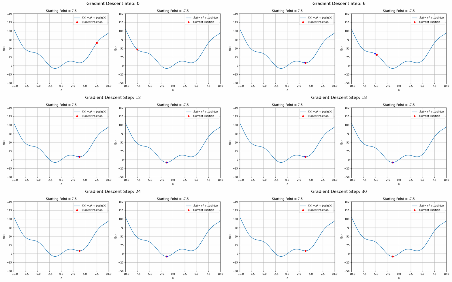
Working with convex functions, gradient descent guarantees finding the function’s global optimum. This is convenient as both the loss functions of a Linear and Logistic Regressions are convex. Unfortunately, a lot of real-world functions are not convex, such as the loss function of complex Neural Networks.
These functions can have local optima in which the gradient descent algorithm could get stuck. See the animation below as an example

Code to generate the animation
import numpy as np
import matplotlib.pyplot as plt
from matplotlib.animation import FuncAnimation

def f(x):
    return x ** 2 + 10 * np.sin(x)

def grad_f(x):
    return 2 * x + 10 * np.cos(x)

def gradient_descent(learning_rate, steps, x_initial):
    x = x_initial
    history = [x]
    for _ in range(steps):
        grad = grad_f(x)
        x = x - learning_rate * grad
        history.append(x)
    return history

# Parameters
x_initials = [7.5, -7.5]  # Starting points for each test case
steps = 30            # Number of steps
learning_rates = [0.1, 0.1]  # Same learning rate for both cases

# Prepare histories for both starting points
histories = []
for lr, x_init in zip(learning_rates, x_initials):
    history = gradient_descent(lr, steps, x_init)
    histories.append(history)

# Prepare the plot
fig, axes = plt.subplots(1, 2, figsize=(12, 5))
x_vals = np.linspace(-10, 10, 1000)
y_vals = f(x_vals)

# Initialize plots
lines = []
arrows = []
for idx, (ax, x_init) in enumerate(zip(axes, x_initials)):
    ax.plot(x_vals, y_vals, label='$f(x) = x^2 + 10 \sin(x)$')
    line, = ax.plot([], [], 'ro', label='Current Position')
    lines.append(line)
    arrows.append(None)  # Placeholder for arrows
    ax.set_title(f'Starting Point = {x_init}')
    ax.set_xlabel('x')
    ax.set_ylabel('f(x)')
    ax.set_xlim(-10, 10)
    ax.set_ylim(-50, 150)
    ax.legend()
    ax.grid(True)

def animate(i):
    fig.suptitle(f'Gradient Descent Step: {i}', fontsize=16)
    artists = []
    for idx, (line, history, ax) in enumerate(zip(lines, histories, axes)):
        x_current = history[i] if i < len(history) else history[-1]
        y_current = f(x_current)
        line.set_data([x_current], [y_current])
        artists.append(line)

        # Remove previous arrow if exists
        if arrows[idx] is not None:
            arrows[idx].remove()

        # Draw arrow from previous point to current point
        if i > 0:
            x_prev = history[i - 1]
            y_prev = f(x_prev)
            arrow = ax.annotate(
                '',
                xy=(x_current, y_current),
                xytext=(x_prev, y_prev),
                arrowprops=dict(arrowstyle='->', color='blue', lw=1.5),
            )
            arrows[idx] = arrow
            artists.append(arrow)
        else:
            arrows[idx] = None  # No arrow in the first frame

    return artists

ani = FuncAnimation(fig, animate, frames=steps + 1, interval=500, blit=True)

plt.tight_layout()
plt.show()
In these cases, running the gradient descent algorithm from different starting points could be a good strategy.
What to do when we do not have the function or gradient?
Part 1 described a set of problems referred to as “black-box” optimisation. These are problems for which we do not have the definition of the function to optimise, or this function is too complex to be solved analytically or is not differentiable (no gradient…).
Looking at the problem above, it is as if we had to decide the numbers of tables and chairs to produce without having the profit function. We could simply try a quantity this month, observe profits, try another quantity next month, observe profits etc… The only information we have are the combinations we try and their outcome.
These problems are the Computer Science equivalent of finding a needle in a hay stack.
PS: There will be much less maths in the next article. I promise.