Linear Programming: Optimisation at the Edges

Subscribe to my newsletter to hear about my latest posts. No spam, I promise.

---

In continuous optimisation problems, it is impossible to try all combinations. But what if a problem could be solved simply by evaluating the corners of the feasible region? This is exactly what linear programming aims to do.

In the previous parts of this series, we have applied no constraints to the number of tables and chairs produced, allowing it to vary within a positive range. Let’s now assume that the company takes its current machine and employee costs as constant. Production is now constrained by the number of hours of carpentry and varnishing.

The company has a total of $200$ carpentry hours and $300$ varnishing hours. Producing chairs and tables leads to the following costs:

• Chairs: $1$ hour of carpentry, $2$ hours of varnishing
• Tables: $2$ hours of carpentry, $2$ hours of varnishing

Formalising constraints we get:

• Carpentry constraint: $q_c+2q_t\le 200$
• Varnishing constraint: $2q_c+2q_t\le 300$

Let’s specify the prices of each:

• Price per table: $p_t=400$
• Price per chair: $p_c=250$

With respect to these constraints, we are aiming to maximise revenue, defined by the following function (based on the unit prices):

$$R(q_c,q_t)=250q_c+400q_t$$

Assuming that any table or chair produced will be sold (this is a very popular brand).

How can we optimise this without trying all possible combinations?

As both the objective function and the constraints are linear (i.e., their graph is a straight line), we can leverage linear programming to evaluate only a few of the solutions.

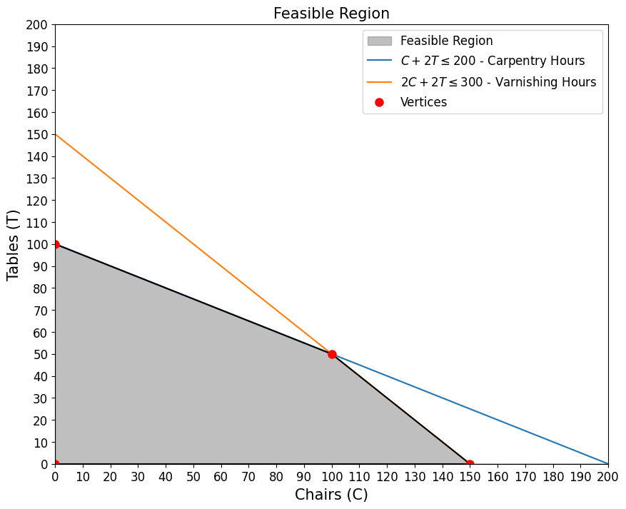
The constraints define the feasible region of the problem, shown in the chart below:

Feasible region

Code to generate the plot

import numpy as np
import matplotlib.pyplot as plt
from scipy.spatial import ConvexHull

# Define the inequalities as functions
def ineq1(C):
    return (200 - C) / 2  # From C + 2T ≤ 200

def ineq2(C):
    return (300 - 2 * C) / 2  # From 2C + 2T ≤ 300

# Objective function for total revenue (for contour plot)
def objective(C, T):
    return 250 * C + 400 * T  # Revenue function

# Generate a grid of C and T values
C = np.linspace(0, 200, 400)
T = np.linspace(0, 200, 400)
C_grid, T_grid = np.meshgrid(C, T)

# Calculate the corresponding T values for each inequality
T1 = ineq1(C)
T2 = ineq2(C)

# Create a mask for the feasible region
ineq1_mask = T_grid <= ineq1(C_grid)
ineq2_mask = T_grid <= ineq2(C_grid)
non_negative_mask = (C_grid >= 0) & (T_grid >= 0)
feasible_region = ineq1_mask & ineq2_mask & non_negative_mask

# Calculate the objective function within the feasible region
Z = objective(C_grid, T_grid)
Z_masked = np.ma.array(Z, mask=~feasible_region)

# Plot the feasible region with contour plot
plt.figure(figsize=(10, 8))
plt.fill_between(C, np.maximum(0, np.minimum(T1, T2)), color='gray', alpha=0.5, label='Feasible Region')


# Plot the lines defining the inequalities
plt.plot(C, T1, label=r'$C + 2T \leq 200$ - Carpentry Hours')
plt.plot(C, T2, label=r'$2C + 2T \leq 300$ - Varnishing Hours')

# Identify and plot the vertices of the feasible region
vertices = np.array([[0, 100], [100, 50], [150, 0], [0, 0]])  # Vertices in (C, T)

# Plot the feasible region boundary
hull = ConvexHull(vertices)
for simplex in hull.simplices:
    plt.plot(vertices[simplex, 0], vertices[simplex, 1], 'k-')

# Plot the vertices
plt.plot(vertices[:, 0], vertices[:, 1], 'ro', markersize=8, label='Vertices')

# Labels and legend
plt.xlabel('Chairs (C)', fontsize=15)
plt.ylabel('Tables (T)', fontsize=15)
plt.xticks(np.arange(0, 201, step=10), fontsize=12)
plt.yticks(np.arange(0, 201, step=10), fontsize=12)
plt.legend(fontsize=12)
plt.title('Feasible Region', fontsize=15)
plt.xlim(0, 200)
plt.ylim(0, 200)
plt.show()

As the constraints are linear, the shape they form is a complex polytope, a pointy shape in a multidimensional space. Most importantly, this shape has corners. Because the objective function is also linear, it will necessarily intersect with the feasible region at one of its corners.

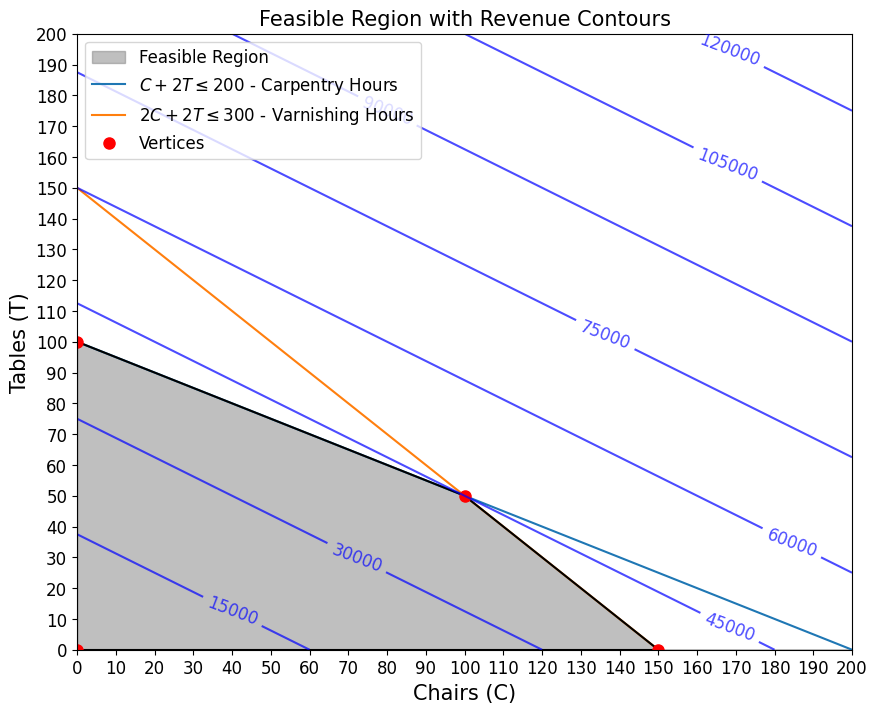
Below is the feasible region with a contour plot of different values of the objective function. As you can see, the intersection of the objective function and the feasible region is at a corner of the feasible region.

Feasible region with revenue contour plot

Code to generate the plot

import numpy as np
import matplotlib.pyplot as plt
from scipy.spatial import ConvexHull

# Define the inequalities as functions
def ineq1(C):
    return (200 - C) / 2  # From C + 2T ≤ 200

def ineq2(C):
    return (300 - 2 * C) / 2  # From 2C + 2T ≤ 300

# Objective function for total revenue (for contour plot)
def objective(C, T):
    return 250 * C + 400 * T  # Revenue function

# Generate a grid of C and T values
C = np.linspace(0, 200, 400)
T = np.linspace(0, 200, 400)
C_grid, T_grid = np.meshgrid(C, T)

# Calculate the corresponding T values for each inequality
T1 = ineq1(C)
T2 = ineq2(C)

# Create a mask for the feasible region
ineq1_mask = T_grid <= ineq1(C_grid)
ineq2_mask = T_grid <= ineq2(C_grid)
non_negative_mask = (C_grid >= 0) & (T_grid >= 0)
feasible_region = ineq1_mask & ineq2_mask & non_negative_mask

# Calculate the objective function within the feasible region
Z = objective(C_grid, T_grid)
Z_masked = np.ma.array(Z, mask=~feasible_region)

# Plot the feasible region with contour plot
plt.figure(figsize=(10, 8))
plt.fill_between(C, np.maximum(0, np.minimum(T1, T2)), color='gray', alpha=0.5, label='Feasible Region')


# Plot the lines defining the inequalities
plt.plot(C, T1, label=r'$C + 2T \leq 200$ - Carpentry Hours')
plt.plot(C, T2, label=r'$2C + 2T \leq 300$ - Varnishing Hours')

# Identify and plot the vertices of the feasible region
vertices = np.array([[0, 100], [100, 50], [150, 0], [0, 0]])  # Vertices in (C, T)

# Plot the feasible region boundary
hull = ConvexHull(vertices)
for simplex in hull.simplices:
    plt.plot(vertices[simplex, 0], vertices[simplex, 1], 'k-')

# Plot the vertices
plt.plot(vertices[:, 0], vertices[:, 1], 'ro', markersize=8, label='Vertices')

# Add contour plot for the objective function
contours = plt.contour(C, T, Z, levels=10, colors='blue', alpha=0.7,label="Objective function")
plt.clabel(contours, inline=True, fontsize=12, fmt='%1.0f')

# Labels and legend
plt.xlabel('Chairs (C)', fontsize=15)
plt.ylabel('Tables (T)', fontsize=15)
plt.xticks(np.arange(0, 201, step=10), fontsize=12)
plt.yticks(np.arange(0, 201, step=10), fontsize=12)
plt.legend(fontsize=12)
plt.title('Feasible Region with Revenue Contours', fontsize=15)
plt.xlim(0, 200)
plt.ylim(0, 200)
plt.show()

From this observation, there is no need to evaluate all combinations; one simply has to evaluate the corners of the feasible region.

To identify the corners of the feasible region, we consider the constraints:

• Carpentry hours: $q_c+2q_t\le 200$
• Varnishing hours: $2q_c+2q_t\le 300$
• Non-negativity: $q_c\ge 0$, $q_t\ge 0$

Solving these constraints, we find the vertices (corners) of the feasible region:

1. Origin point: $(q_c,q_t)=(0,0)$

2. At $q_t=0$:

• From the carpentry constraint: $q_c\le 200$
• From the varnishing constraint: $2q_c\le 300⟹q_c\le 150$
• The more restrictive is $q_c\le 150$, so we have the point $(q_c,q_t)=(150,0)$

3. At $q_c=0$:

• From the carpentry constraint: $2q_t\le 200⟹q_t\le 100$
• From the varnishing constraint: $2q_t\le 300⟹q_t\le 150$
• The more restrictive is $q_t\le 100$, so we have the point $(q_c,q_t)=(0,100)$

4. Intersection point of the two constraints:

• From the carpentry constraint: $q_c=200-2q_t$
• Substitute into the varnishing constraint: $$2(200-2q_t)+2q_t\le 300$$ Simplify: $$\begin{array}{rl}400-4q_t+2_{q}t& \le 300\\ 200-q_t& \le 150\\ q_t& \ge 50\end{array}$$ Substitute $q_t=50$ back into $q_c=200-2q_t$: $$q_c=200-2\times 50=100$$ So the intersection point is $(q_c,q_t)=(100,50)$

Therefore, the corners of the feasible region are at:

• $(0,0)$
• $(150,0)$
• $(0,100)$
• $(100,50)$

We then evaluate the objective function at each corner:

• At $(0,0)$: $$R=250\times 0+400\times 0=\mathrm{\$}0$$

• At $(150,0)$: $$R=250\times 150+400\times 0=\mathrm{\$}37500$$

• At $(0,100)$: $$R=250\times 0+400\times 100=\mathrm{\$}40000$$

• At $(100,50)$: $$R=250\times 100+400\times 50=\mathrm{\$}45000$$

The maximum revenue occurs at $(q_c,q_t)=(100,50)$, with revenue of $\mathrm{\$}45000$.

This type of shortcut is only possible when both the objective function and the constraints are linear.

This may still seem abstract when talking about chairs and tables. But many other problems can also be solved using the same framework:

• Scheduling matinenance staff shifts in a hotel
• Combination of raw materials in industrial food production
• Machine time allocation in a factory

Final Thoughts

The efficiency of linear programming reminds us that the more information we have about a problem, the less computation we need to solve it. This information about the problem (meta-information) can be leveraged to devise smart algorithms taking shortcuts.

But what happens when you cannot make any assumptions? What if you can only observe the output of the objective function? If this sounds exciting, head over to this series’ next post on black-box optimisation problems.

Other Articles in this Series

• Getting the intuition of optimisation
• Little by litte: Optimising function with analysis and gradient descent
• Black-box Optimisation: Searching in the Dark
• Multi-fidelity Optimisation: The art of skimming