Big Oh, Big Omega, Big Theta: What is asymptotic notation?

Computer Scientists use asymptotic notation is to bind algorithmic complexity expressed as a function of its input size. Instead of focussing on a function’s exact definition (e.g., \(f(x) = 2x + 3\)), these functions are discussed in terms of their upper and lower bounds.

Where the previous part of this series focused on the intuition behind algorithm complexity using the example of a party’s organisation, this article will focus on rigorously analysing the run time of an algorithm using asymptotic notation. It will uncover the meaning of characters like \(O\), \(\Omega\), and \(\Theta\). By the end of this article, you will be able to describe the growth rate of an algorithm’s runtime as its input grows infinitely large.

Binding f(n) with O(n) and Omega(n)

The first step of rigorous analysis is to express the runtime of an algorithm as a function of \(n\), its input size. Following the party example, the time complexity of greeting all guests can be defined as the function \(f(n) = n\); as each new guest requires a new greeting. If greetings include both “Hello” and “Goodbye” for each guest, it would then be defined as \(f(n) = 2n\); as each guest requires at least two interactions.

Quick Exercise

1. What would be the time complexity of this last greeting function if \(\frac{1}{3}\) of the guests leave without saying goodbye?
   
2. More generally, what if an arbitrary ratio \(\alpha\) leave without saying goodbye?
   
3. What if \(\alpha\) of guests leave without saying goodbye and \(\beta\) of guests enter without saying “hi”? With both \(\alpha\) and \(\beta\) real numbers between 0 and 1.

Expand to view answers

Answers:
a) \(f(n) = n + \frac{2}{3} n = \frac{5}{3} n\)
b) \(f(n) = n + (1-\alpha)n = n(2 - \alpha)\)
c) \(f(n) = (1-\beta)n + (1-\alpha)n = n(2 - \alpha - \beta)\)

Now that the algorithm runtime is represented as a function of its input, we can start binding its run time as its input size grows toward infinity. This is where Big O comes in, along with our first Big Formula Warning.

Mathematical shortcut

Are you only interested in quickly finding the \(O\) upper-bound of a function without getting into the weeds of asymptotic notation? If yes, there is a shortcut. Let’s say you want to know the upper-bound complexity of the function \(f(n)=2n^2 + n + 2\). You can identify the fastest growing term (\(n^2\)), drop any constant multiplied to it (2) and you will get complexity \(O(n^2)\).

To understand why this works and the meaning of the characters \(O\), \(\Omega\) and \(\Theta\), read on.

Binding functions with \(O\) (pronounced “Big-Oh”)

A function \(f(n)\) is said to be \(O(g(n))\) if and only if: \(f(n) \leq c \cdot g(n)\) for all \(n \subseteq \mathbb{N}\), with \(n > n_0\) and \(c \subseteq \mathbb{R}^+\).

Let’s reword this in plain English.

• \(f(n)\) is the algorithm’s run time as a function of \(n\), the input size
• \(g(n)\) is the function by which we are trying to bind \(f(n)\), in this case, our candidate upper bound. Remembering the example explained in part 1, the task of greeting all guests had an upper-bound time complexity of \(O(n)\). In this case, \(g(n) = n\). Other \(g(n)\)’s studied were \(n^2\), \(\log(n)\) and \(2^n\)
• \(c\) is any positive real number that does not depend on \(n\) (e.g., 2 or 65.3, but not \(2n\))
• \(n_0\) is the starting point arbitrarily chosen, usually set to a number making algorithm analysis easier (e.g., \(n_0 = 2\) for expressions using logs).

In English, the statement \(f(n) = O(n)\) means that \(f(n)\) asymptotically grows no faster than \(n\). “Asymptotically” refers to the fact that \(n\) grows towards infinity. The “no faster” stems from the upper-bound calculated in the expression \(f(n) \leq c \cdot g(n)\).

Let’s imagine that a party’s organisation only requires setting up the house, greeting all guests and cleaning up. Let’s also assume that setting up and cleaning up take \(100\) minutes each, regardless of the number of guests (bold assumption). We will also assume that greeting a guest takes one minute, saying goodbye takes another minute.

What would be \(f(n)\) the total time required to organise the party in minutes, with \(n\) the number of guests?

\[ f(n) = 2 \cdot 100 + 2n = 200 + 2n \]

Now, what is the asymptotic upper-bound of this expression?

An easy mathematical shortcut there is to take the fastest growing term (here \(2n\)), drop the constant (here \(2\)), and you will get the asymptotic upper bound (here \(n\)). No more than this. But why does this work? The answer lies in the mathematical formulation of asymptotic notation.

Let’s try to prove this intuition by proving the following: \(f(n) \leq c \cdot g(n)\) for all \(n \subseteq \mathbb{N}\), with \(n > n_0\) and \(c \subseteq \mathbb{R}^+\).

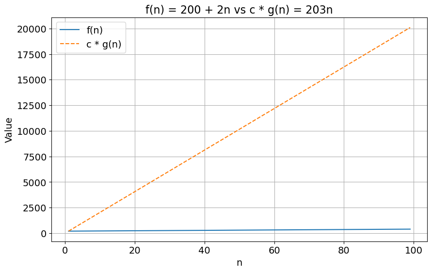
With \(f(n) = 200 + 2n\) and \(g(n) = n\). The goal is to find a constant \(c\) and a starting point \(n_0\) so that the condition \(f(n) \leq c \cdot g(n)\) holds. One could simply set \(c = 203\) and \(n_0 = 1\). This would yield the following condition

\[f(n) \leq 203 \cdot n\] \[200 + 2n \leq 203n, \forall n \geq n_0 \implies f(n)=O(n)\]

The two sides of this inequality can be visualised in the chart below:

Code to generate plot

import matplotlib.pyplot as plt
import numpy as np

n = np.arange(1, 100)
f_n = 200 + 2 * n
g_n = 203 * n

plt.figure(figsize=(10, 6))
plt.plot(n, f_n, label='f(n)')
plt.plot(n, g_n, label='c * g(n)', linestyle='--')
plt.xlabel('n', fontsize=14)
plt.ylabel('Value', fontsize=14)
plt.title('f(n) = 200 + 2n vs c * g(n) = 203n', fontsize=16)
plt.legend(fontsize=14)
plt.xticks(fontsize=14)
plt.yticks(fontsize=14)
plt.grid(True)
plt.show()

Is \(f(n) = 200 + 2n\) expression also \(O(n^2)\)? To answer this, let’s remember our English interpretation. If \(f(n)\) is \(O(n^2)\), it means that \(f(n)\) grows asymptotically no faster than \(n^2\). Which does sound correct, as \(n\) grows slower than \(n^2\).

Let’s prove this using the formula \(f(n) \leq c \cdot g(n)\).

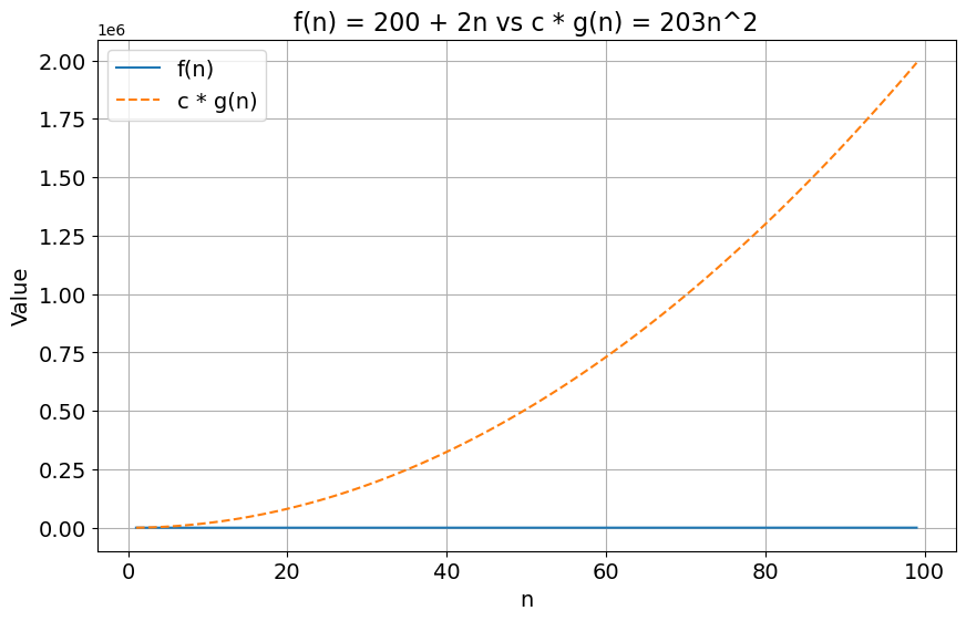
With \(c = 203\) and \(n_0 = 1\), the condition still holds: \[ 200 + 2n \leq 203 \cdot n^2, \forall n \geq n_0 \]

Job done! \(f(n)\) is also of time complexity \(O(n^2)\).

The difference of growth rate between \(n\) and \(n^2\) can be visualised in the plot below:

Code to generate plot

import matplotlib.pyplot as plt
import numpy as np

n = np.arange(1, 100)
f_n = 200 + 2 * n
g_n2 = 203 * n**2

plt.figure(figsize=(10, 6))
plt.plot(n, f_n, label='f(n)')
plt.plot(n, g_n2, label='c * g(n)', linestyle='--')
plt.xlabel('n', fontsize=14)
plt.ylabel('Value', fontsize=14)
plt.title('f(n) = 200 + 2n vs c * g(n) = 203n^2', fontsize=16)
plt.legend(fontsize=14)
plt.xticks(fontsize=14)
plt.yticks(fontsize=14)
plt.grid(True)
plt.show()

Any function with upper bound \(O(n)\) is also \(O(n^2)\). This may sound counterintuitive as a single question appears to have multiple answers. Let’s remember that we are looking for an upper bound. A function with upper-bound \(O(n)\) will also have upper-bound \(O(n^2)\). The computer scientist’s job will be to find the tightest upper-bound possible, i.e., the smallest upper-bound.

A function of complexity \(O(n)\) will also be of complexity \(O(n \cdot \log(n))\), \(O(n^2)\), \(O(2^n)\), \(O(n!)\). When analysing functions, it is important to keep the following order of complexities in mind:

\[ 1 < \log(n) < n < n \cdot \log(n) < n^2 < 2^n < n! \]

A function of a given upper-bound complexity will also have all faster growing functions as upper-bound. As an example, a function of complexity \(O(\log(n))\) is also \(O(n)\).

Note on \(O(1)\)

An algorithm runs in constant time or complexity \(O(1)\) when its runtime does not depend on the size of the input. Sticking to the party example, if the only tasks required for a party are to prepare and clean up, and none of these depend on the number of guests, we get \(f(n) = 200\). As 200 is a constant (it does not depend on any variable), \(f(n) = 200 = O(1)\).

Expanding to Big-Omega (\(\Omega\)) and Big-Theta (\(\Theta\))

Big-Omega (\(\Omega\)) is very similar to Big-Oh (\(O\)), but instead of being an upper-bound, it is a lower-bound. In mathematical terms, instead of looking for a \(c\) and \(g(n)\) satisfying the upper-bound condition \(f(n) \leq c \cdot g(n)\), we try to satisfy the lower bound condition \(f(n) \geq c \cdot g(n)\).

What would be the asymptotic lower bound of \(f(n) = 200 + 2n\)?

Here again, the trick of identifying the fastest growing term (\(2n\)) and dropping the constant would give us a lower-bound \(\Omega(n)\). The reason this is correct will be explained below.

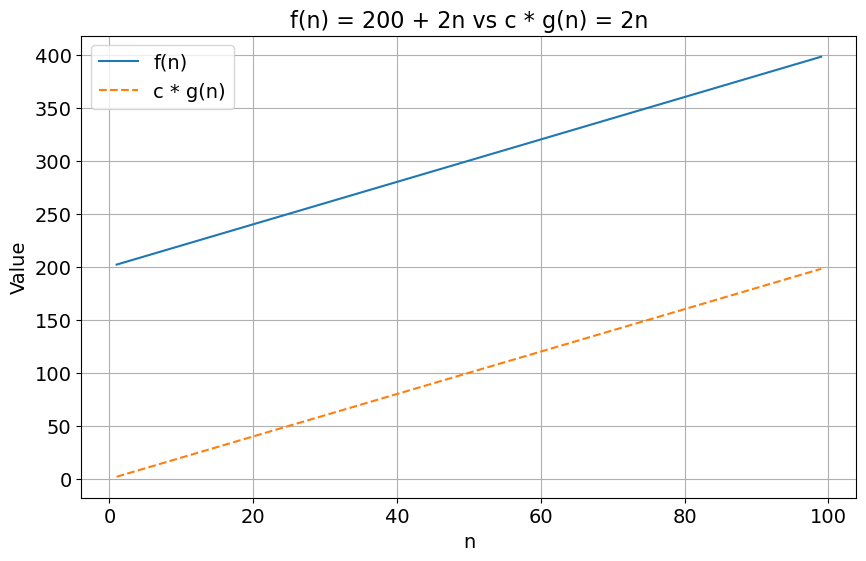
Using \(n_0 = 1\) and \(c = 2\), we get \(200 + 2n \geq 2n\). The condition is satisfied and \(f(n)\) is \(\Omega(n)\)! We can validate this finding by plotting both sides of this inequality below.

Code to generate plot

import matplotlib.pyplot as plt
import numpy as np

n = np.arange(1, 100)
f_n = 200 + 2 * n
g_omega_n = 2 * n

plt.figure(figsize=(10, 6))
plt.plot(n, f_n, label='f(n)')
plt.plot(n, g_omega_n, label='c * g(n)', linestyle='--')
plt.xlabel('n', fontsize=14)
plt.ylabel('Value', fontsize=14)
plt.title('f(n) = 200 + 2n vs c * g(n) = 2n', fontsize=16)
plt.legend(fontsize=14)
plt.xticks(fontsize=14)
plt.yticks(fontsize=14)
plt.grid(True)
plt.show()

To test your understanding, try to answer the following questions:

1. Is \(f(n) = 200 + 2n\) also \(\Omega(n^2)\)?
2. Is \(f(n) = 200 + 2n\) also \(\Omega(\log(n))\)?

Expand to see the answers

Answers

1. No it is not. Because there is no constant \(c\) and integer \(n_0\) so that \(200 + 2n \geq c \cdot n^2\) is satisfied as \(n\) grows to infinity.
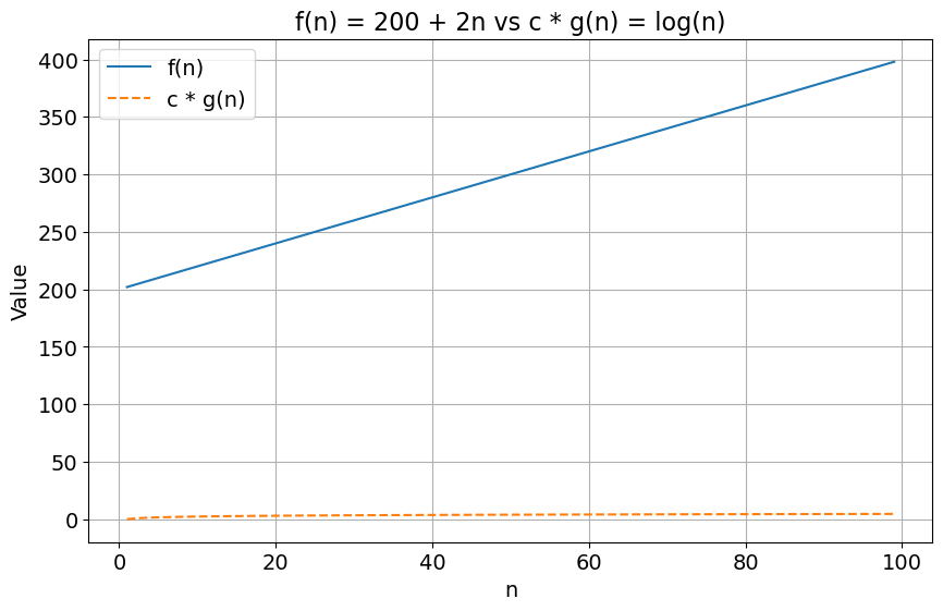
2. Yes, as \(\log(n)\) grows much slower than \(n\). As an example, using \(n_0 = 2\) and \(c = 1\), we get \(200 + 2(n) > \log(n)\), which satisfies the condition for all \(n > n_0\). See the chart below.

Code to generate plot

import matplotlib.pyplot as plt
import numpy as np

n = np.arange(1, 100)
f_n = 200 + 2 * n
g_log_n = np.log(n)

plt.figure(figsize=(10, 6))
plt.plot(n, f_n, label='f(n)')
plt.plot(n, g_log_n, label='c * g(n)', linestyle='--')
plt.xlabel('n', fontsize=14)
plt.ylabel('Value', fontsize=14)
plt.title('f(n) = 200 + 2n vs c * g(n) = log(n)', fontsize=16)
plt.legend(fontsize=14)
plt.xticks(fontsize=14)
plt.yticks(fontsize=14)
plt.grid(True)
plt.show()

A function with a lower-bound \(\Omega(n)\) will also have a lower-bound of \(\Omega(log(n))\) and \(\Omega(1)\). You can use the following order as reference (same as above). The Computer Scientist’s job is to find the tightest lower-bound possible, i.e., the highest lower-bound.

\[ 1 < \log(n) < n < n \cdot \log(n) < n^2 < 2^n < n! \]

Big-Theta (\(\Theta\)) represents the tightest bound of a function’s growth rate. For a function \(f(n)\) to be of complexity \(\Theta(g(n))\), it has to satisfy the following condition: \(c_1 \cdot g(n) \geq f(n) \geq c_2 \cdot g(n)\) with \(c_1\) and \(c_2\) two constants. In other words, it has to satisfy both the lower-bound and the upper-bound condition.

When the function studied is mathematically defined, e.g., \(f(n) = 200 + 2n\), the trick of identifying the fastest growing term and dropping the constant still works. Here, \(f(n) = \Theta(n)\).

As an exercise, try proving this by finding constants \(c_1\) and \(c_2\) with \(n_0 = 1\).
Hint: it is not harder than finding the upper- and lower-bound of the function.

By setting \(c_1 = 203\) and \(c_2 = 1\), we get the following set of inequalities which hold for all \(n > n_0\):

\[ 203 \cdot n > 200 + 2n > 1 \cdot n \]

To test your understanding, try answering the following questions:

1. Is this \(f(n)\) also \(\Theta(n^2)\)?
2. Is it also \(\Theta(\log(n))\)?

Expand to see the answers

Answers

1. No, as there is no \(c\) and \(n_0\) such that \(200 + 2n \geq c \cdot n^2\) for all \(n > n_0\).
2. Similarly, there is no \(c\) and \(n_0\) such that \(200 + 2n \leq c \cdot \log(n)\) for all \(n > n_0\). If in doubt, plot both sides of the equation or try plugging large numbers into the formula.

Final Thoughts

Big-Oh (\(O\)), Big Omega (\(\Omega\)), and Big Theta (\(\Theta\)) are indispensable tools to analyse the complexity of algorithms. They allow us to abstract away from the specifics of an algorithm by describing its growth rate. This then allows us to select the algorithm best suited for the problem at hand.

Now that we understand the theory behind asymptotic notation, the following part of this series will apply this knowledge to study the complexity of Python code snippets.

Related Articles

• What is algorithm complexity?
• How to analyse the complexity of a Python code snippet?