What is the Complexity of Euclid’s Algorithm?
Euclid’s algorithm is one of the earliest algorithms ever recorded. It finds the Greatest Common Divisor or “GCD” between two integers \(a\) and \(b\) with \(a > b\). As an example, the GCD of \(36\) and \(27\) is \(9\) as it is the largest integer that divides both numbers.
One simple way to find this GCD is to iterate over all integers between \(1\) and \(b\) (the lowest of the two) and find the largest one dividing both \(a\) and \(b\). This brute force approach is of complexity \(O(b)\).
Euclid’s algorithm elegantly leverages the fact that the GCD of two numbers is also the GCD of their difference to significantly reduce computation time.
Starting from our intuition, this must be better than the brute force method \(O(b)\), but how much exactly?
Let \(a_0 = a\) and \(b_0 = b\).
In the following update, \(a_1 = b_0\) and \(b_1 = a_0 \mod b_0\).
More generally, \(a_{k+1} = b_k\) and \(b_{k+1} = a_k \mod b_k\).
Using the properties of the modulo operator, it can be proven that \(b_{k+2} \leq \frac{b_k}{2}\). In English, that b will more at least be divided by 2 after two steps of Euclid’s algorithm.
Quickly validating this with a quick example, with \(a_0 = 72\) and \(b_0 = 54\):
\(a_1 = 54, b_1 = 72 \mod 54 = 18\)
\(a_2 = 18, b_2 = 54 \mod 18 = 0\)
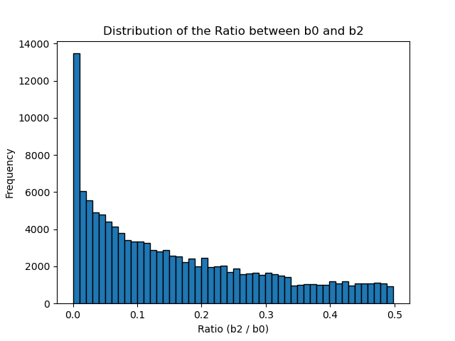
The proof is beyond the scope of this article (see Appendix for a proof), but this finding can be empirically validated by computing \(b_0\) and \(b_2\) for all combinations of \(a\) and \(b\) within the range \([1, 500]\) and plotting their ratio.
Computer Simulation

Python code used to generate the chart
import matplotlib.pyplot as plt

def euclid_algorithm(a, b):
    b0 = b
    a1 = b
    b1 = a % b
    if b1 == 0:
        return b0, None
    a2 = b1
    b2 = a1 % b1

    return b0, b2

ratios = []

for a in range(1, 501):
    for b in range(1, 501):
        if a > b:
            b0, b2 = euclid_algorithm(a, b)
            if b2 is not None:
                ratio = b2 / b0
                ratios.append(ratio)

plt.hist(ratios, bins=50, edgecolor='black')
plt.xlabel('Ratio (b2 / b0)')
plt.ylabel('Frequency')
plt.title('Distribution of the Ratio between b0 and b2')
plt.show()
Achieving Logarithmic Upper-Bound
Given the fact the upper-bound \(b_{k+2} \leq \frac{b_k}{2}\), we can show that the time complexity of Euclid’s algorithm is \(O(log(n))\).
Using our Computer Science intuition, the division by 2 points to a logarithmic decrease.
As \(b\) is divided by 2 every two steps, we need to find the number of steps needed (\(k\)) to get \(b \leq 1\).
Putting this into mathematical form, we get:
\(\frac{b_0}{2^{k/2}} = 1\)
\(2^{k/2} = b_0\)
\(\frac{k}{2} = \log(b_0)\)
\(k = 2 \log(b_0) \implies O(\log(b))\)
Final Thoughts
In its beautiful simplicity, Euclid’s algorithm is a prime example of leveraging information about a problem to avoid exhaustive search. By exploiting the fact that two numbers’ Greatest Common Divisor is also the Greatest Common Divisor of their difference, this algorithm recursively reduces the problem - reaching a time complexity of \(O(\log(b))\).
Appendix
Proving \(b_{k+2} \leq \frac{b_k}{2}\)
Before going into further details, let’s remember how Euclid’s algorithm works with the example of \(a_0 = 72\) and \(b_0 = 54\).
We can summarise the steps in the following table:
| Step Number | \(a\) | \(b\) |
|---|---|---|
| 0 | 72 | 54 |
| 1 | 54 | 18 |
| 2 | 18 | 0 |
The update rule of Euclid’s algorithm is as follows:
\[ \begin{cases} a_{k+1} = b_k \\ b_{k+1} = a_k \mod b_k \end{cases} \]
Now, how to prove that \(b_{k+2}\) is always less than \(\dfrac{b_k}{2}\)? There are two cases to study:
Case 1: \(b_{k+1} < \dfrac{b_k}{2}\)
In this case, \(b_{k+1}\) is already less than \(\dfrac{b_k}{2}\). This is the case at the first update of the example above, with \(b_0 = 54\) and \(b_1 = 18\).
Case 2: \(b_{k+1} > \dfrac{b_k}{2}\)
We observe the following:
\[ b_{k+1} = a_k \mod b_k \tag{1} \]
\[ b_{k+2} = b_k \mod b_{k+1} \tag{2} \]
If \(b_{k+1} > \dfrac{b_k}{2}\), then:
\[ b_k \mod b_{k+1} = b_k - b_{k+1} \tag{3} \]
This is due to the division rule of the quotient and remainder:
\[ b_k = b_{k+1} \times 1 + (b_k - b_{k+1}) \]
So, the remainder is \(b_k - b_{k+1}\).
Substituting equation \((3)\) into equation \((2)\), we get:
\[ b_{k+2} = b_k - b_{k+1} \tag{4} \]
From \(b_{k+1} > \dfrac{b_k}{2}\), we have:
\[ b_k - b_{k+1} < b_k - \dfrac{b_k}{2} = \dfrac{b_k}{2} \]
Substituting back into equation \((4)\), we obtain:
\[ b_{k+2} < \dfrac{b_k}{2} \tag{5} \]
Thus, in both cases, we have shown that \(b_{k+2} < \dfrac{b_k}{2}\).