Saved by Data Structures: Digging into Nearest Neighbours

It was 8pm, I was sleep-deprived, and all I could hear was the roar of my Intel Core i5 CPU, without any results in sight. Little did I know that data structures would allow me to get these results in seconds.

This was summer 2020. I was still starting out as a Data Science consultant and had been working on a demanding project for a pharmaceutical company, my first experience in pricing. Before this project, the firm had to review the price of roughly 1000 different SKUs (Stock Keeping Units, i.e., distinct products) every month. They usually did this as a product review meeting, generally lasting around 12 hours (just to put your next meeting in perspective).

My task was to build a Data Science solution to improve the efficiency of that process. This is not an easy task as we could only observe transactions and not demand. When the product was not in stock, a common occurrence in this market, we could not observe the transactions that would have happened had we had stock.

My first intuition was to detect unusual market situations and flag them to the product review team. Such situations could include competitors going out of stock or demand spikes due to exogenous market factors. In this situation, it would be in the company’s interest to raise prices before selling all remaining inventory (the moral implications of this were not lost on my 22-year-old self).

One could think: this is an easy supervised learning task, let’s just find all of our demand spikes in the database and train a Machine Learning model to predict them. The issue was, these labels did not exist. I did come up with a way to label the dataset, but that is not what I want to write about today.

We did not have labels (dataset records saying: “this is a high demand situation!!”), but the management and sales teams kept telling us their stories of this drug selling out quickly in April 2018 or this other missed opportunity in June of last year. I was convinced that we could make the most of this limited information.

From Anecdotes to Vectors

Then, one morning, I thought: What if we represented each situation, a combination of product and point in time (e.g., paracetamol in April 2019), as a vector, or point in a high-dimensional space?

Well, well, this article escalated quickly… Let me explain this in English. Each situation has data associated with it: sales in the previous week, number of transactions in the previous weeks, number of distinct customers, etc.

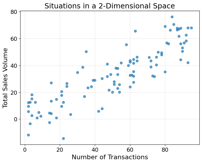
As a hypothetical example, you can use this data to represent each situation in space. In the chart below, I show a simplified example in which each situation is represented in a two-dimensional space: number of transactions and total sales volume.

Visualising situations in a 2-dimensional space

Code used to generate the plot

import numpy as np
import matplotlib.pyplot as plt

np.random.seed(42)
# this data is used later in the article
x = np.random.randint(1, 100, 100)
y = (x * 0.3 + np.random.normal(0, 5, 100))*2.2

plt.figure(figsize=(8, 6))
plt.scatter(x, y, alpha=0.7)
plt.title("Situations in a 2-Dimensional Space", fontsize=18)
plt.xlabel("Number of Transactions", fontsize=16)
plt.ylabel("Total Sales Volume", fontsize=16)
plt.xticks(fontsize=14)
plt.yticks(fontsize=14)
plt.grid(alpha=0.3)
plt.show()

This intuition can be extended to many more dimensions, such as the number of customers, sales in the previous week, etc. Be careful though, you may hit the curse of dimensionality if you include too many, but that is another blog post in itself.

Representing things such as events, products, words, or documents as vectors is a habit of Machine Learning practitioners. It helps us convert things in the world into lists of numbers. We can then apply operations on these vectors to solve tough problems and bring the solution back into the real world. This is the material for yet another post, let’s not get sidetracked.

Getting back to our example, we now have each situation, product and point in time, represented in a high-dimensional space.

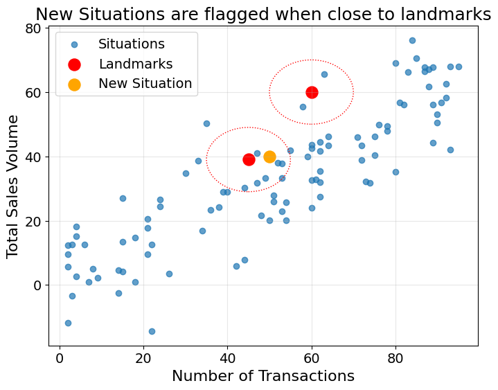
We know from the stories of the company’s sales team that some of these situations or points in space represent high demand situations. We could use these as landmarks, and any time a new situation comes close to these landmarks, we would flag it to the product review team.

Landmarks and new situations in space

Code used to generate the plot

import numpy as np
import matplotlib.pyplot as plt
from sklearn.neighbors import NearestNeighbors

data = np.column_stack((x, y))

landmarks = np.array([[60,60], [45,39]])
new_point = np.array([[50, 40]])

# Fit nearest neighbours
nbrs = NearestNeighbors(n_neighbors=1).fit(data)
distances, indices = nbrs.kneighbors(new_point)

# Plot
plt.figure(figsize=(8, 6))
plt.scatter(data[:, 0], data[:, 1], alpha=0.7, label="Situations")
plt.scatter(landmarks[:, 0], landmarks[:, 1], color="red", s=150, label="Landmarks")
plt.scatter(new_point[:, 0], new_point[:, 1], color="orange", s=150, label="New Situation")

for landmark in landmarks:
    circle = plt.Circle(landmark, radius=10, color="red", linestyle="dotted", fill=False)
    plt.gca().add_artist(circle)

# Add labels and legend
plt.legend(fontsize=14)
plt.title("New Situations are flagged when close to landmarks", fontsize=18)
plt.xlabel("Number of Transactions", fontsize=16)
plt.ylabel("Total Sales Volume", fontsize=16)
plt.xticks(fontsize=14)
plt.yticks(fontsize=14)
plt.grid(alpha=0.3)
plt.show()

Here, the new situation (orange point) would be flagged as “situation of interest” as it is close to one existing landmark.

Finding Nearest Neighbours

Eureka, great idea, job done. Or so you would think.

I now had to find a way to query the nearest neighbour of each new situation and find out if a landmark was part of these neighbours.

To test this out, I wrote a quick script to get the 10 nearest neighbours of each situation in our dataset. This would be done in minutes and I could go to bed, getting the sleep I direly needed.

As a quick review, you can get the distance between two points in space using the Euclidean distance, a generalisation of the Pythagorean theorem over \(n\) dimensions. \[ d(x, y) = \sqrt{\sum_{i=1}^n (x_i - y_i)^2} \]

In two dimensions, \(n\) would equal \(2\) and the formula would look like:

\[ \sqrt{(x_1 - y_1)^2 + (x_2 - y_2)^2} \]

This extends to higher dimensions with higher values of \(n\).

Yet, the laws of Computer Science destroyed my plan. There was no way my laptop would, for every one of the 300,000 situations (drug/point in time), calculate the distance to every other situation and pick the closest 10. I could vectorise my code however I wanted, there was no way to do this over the dimensions of my dataset (number of columns).

How to get around this? Luckily, as was the case with most things in my career, some people had already figured it out. I recalled my Algorithms and Data Structures course and realised: wait, there was more information I could leverage to solve this problem. Nothing forced me to store my data as a list. With this list approach, I would be forced to compute the distance between each situation and every other. This is clearly inefficient as I know from the start that some of these are very far away in the feature space.

What if I stored my data as a tree? Stay with me there. What if I stored my data based on the values within its data vector? Then, I would only have to compute a handful of distances to get the nearest neighbours I needed.

This approach is called a k-d tree (“k-dimensional tree”). It is a data structure that organises data into a partition of a k-dimensional space.

Stylised representation of a K-D tree

This data structure is particularly useful to find nearest neighbours of points in \(O(\log(n))\), much quicker than my \(O(n^2)\) list-based madness. If you find this notation intimidating and want to learn more about algorithmic complexity, head to my series on the topic, else read on. The aim of this paragraph is only to show that my initial approach was theoretically doomed.

With this in mind, I used scipy’s KDTree to build a tree and query it to get each situation’s closest neighbours. The script ran in less than a minute. Hallelujah! After a quick visual check of the results, I fell asleep.

The next morning, I presented my idea to my manager and client, and they all liked it. The project could continue.

Runtime comparison

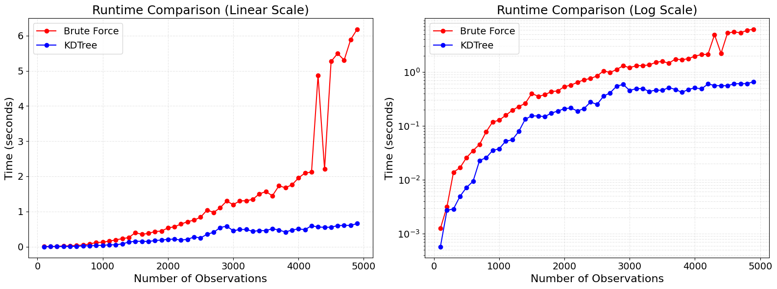
But how much better is the KD-tree approach compared to the brute force approach? Well, much better. The chart below shows the runtime of both methods as the input size grows from 100 to 5000. The KD-tree approach is an order of magnitude faster.

Runtime comparison of the two approach, KD-tree performs an order of magnitude better

Code used to generate the plot

import numpy as np
import matplotlib.pyplot as plt
import time
from scipy.spatial import KDTree

dataset_sizes = np.arange(100, 5000, 100)

brute_force_times = []
kdtree_times = []

for size in dataset_sizes:
    data = np.random.rand(size, 30)
    
    # Brute force approach
    start = time.time()
    distances = np.linalg.norm(data[:, None] - data, axis=2)
    end = time.time()
    brute_force_times.append(end - start)
    
    # KDTree approach
    start = time.time()
    tree = KDTree(data)
    nearest = tree.query(data, k=10)
    end = time.time()
    kdtree_times.append(end - start)

fig, axes = plt.subplots(1, 2, figsize=(16, 6))

axes[0].plot(dataset_sizes, brute_force_times, label="Brute Force", color="red", marker="o", linestyle="-")
axes[0].plot(dataset_sizes, kdtree_times, label="KDTree", color="blue", marker="o", linestyle="-")
axes[0].set_title("Runtime Comparison (Linear Scale)", fontsize=18)
axes[0].set_xlabel("Number of Observations", fontsize=16)
axes[0].set_ylabel("Time (seconds)", fontsize=16)
axes[0].grid(alpha=0.3, linestyle="--")
axes[0].legend(fontsize=14)
axes[0].tick_params(axis="both", labelsize=14)

axes[1].plot(dataset_sizes, brute_force_times, label="Brute Force", color="red", marker="o", linestyle="-")
axes[1].plot(dataset_sizes, kdtree_times, label="KDTree", color="blue", marker="o", linestyle="-")
axes[1].set_title("Runtime Comparison (Log Scale)", fontsize=18)
axes[1].set_xlabel("Number of Observations", fontsize=16)
axes[1].set_ylabel("Time (seconds)", fontsize=16)
axes[1].set_yscale("log")  # Log scale for runtime
axes[1].grid(alpha=0.3, which="both", linestyle="--")
axes[1].legend(fontsize=14)
axes[1].tick_params(axis="both", labelsize=14)

plt.tight_layout()
plt.show()

Note: I would have liked to continue this comparison with a higher sample size, but my Mac M1 CPU was not liking it. I decided to stop at 5000. The \(O(n^2)\) complexity of the brute force approach was too much for my laptop.

Some implementation details

To implement this, we can start by generating a random dataset with 1000 rows and 30 columns (also referred to as “dimensions”). This can be done using numpy:

import numpy as np

data = np.random.rand(1000, 30) # 1000 rows, 30 columns

To implement the brute force method, we could compute the distance of each row to every other row using a nested loop:

distances = np.zeros((1000, 1000))
for i in range(1000):
    for j in range(1000):
        distances[i, j] = np.linalg.norm(data[i] - data[j])

The np.linalg.norm function computes the Euclidean distance between two vectors in an efficient way.

Note: as a rule thumb, your intuition should tell you that something is wrong when you hear the words “nested loops”. It is rarely a good sign.

As always in numerical computation in Python, there is usually a smart way to avoid nested loops using numpy. It would look something like this:

distances = np.linalg.norm(data[:, None] - data, axis=2)

This computes the distance between each row and every other row in a vectorized way. The output is a 1000x1000 matrix in which eaach element (\(i\),\(j\)) is the distance between row \(i\) and row \(j\).

This method is already much faster, but still grows with complexity \(O(n^2)\).

Now let’s turn to KD-trees. We can use the scipy.spatial.KDTree implementation to build a KD-tree with our data and query the nearest neighbours of each observation:

from scipy.spatial import KDTree

tree = KDTree(data)
nearest = tree.query(data, k=10)

That is it.

Now let’s benchmark the above methods for a dataframe of 5000 rows and 30 columns using the timeit framework.

import timeit
import numpy as np
from scipy.spatial import KDTree

data = np.random.rand(5000, 30)

brute_force_time = timeit.timeit(lambda: np.linalg.norm(data[:, None] - data, axis=2), number=10)
kdtree_time = timeit.timeit(lambda: KDTree(data).query(data, k=10), number=10)

print(f"Brute force time: {brute_force_time}") 
# Brute force time: 114.46504104199994
print(f"KD-tree time: {kdtree_time}") 
# KD-tree time: 6.730712166012381

Just below a 20x speed-up. Sometimes, a test is worth more than a thousand words. Again, my CPU did not like this at all.

Final Thoughts

With hindsight and the tools we have now, I would probably do things differently.

We sometimes forget that it is very easy to write terrible code. And when your code is terrible, no additional amount of compute will save you. When developing under pressure, it does not always seem natural to stop and think about data structures to solve a problem in a more efficient way. A good reminder to worry about the way in which we store data.

As I teach my Computer Science students, data storage conditions data usage. This may not be grammatically correct, but it gets the point across. If your bookshelves are sorted, you will be able to find books quicker. If it is a pile, it will be very easy to add books, much harder to retrieve them.

Thinking about the problems you are currently working on, how could you better leverage data structures to build a more efficient solution?