What is a derivative? Building a graphical intuition
But Eliott, what is a derivative?
It was a warm sunny day in Paris, in the summer of 2017. I was tutoring A-level maths to pay for my holidays and also because I really enjoyed both maths and teaching. I thought that I was doing a pretty good job until I was asked the question above.
At that instant, it was the first time I experienced the simple truth: knowing is not sufficient for teaching.
Of course I “knew” what a derivative was. I knew that the derivative of \(x^2\) was \(2x\). I knew the product rule and the chain rule. I had been using derivatives to solve microeconomics optimisation problems.
And yet, at that moment, I could not explain to a 17-year-old what a derivative was. We looked it up together in the book. By the end of the session, we had both learnt a lot. This student, by the way, got a very good grade on her exam.
Eight years later, I am revisiting the concept of derivatives and differentiation in light of my tutoring and lecturing experience, and after 6 years of working as a Data Scientist in industry.
Whether you train Machine Learning models daily, or derivatives are an old (and dreaded) high school memory, there should be something you can take away from this article.
Why should we care about derivatives?
The world around us changes all the time. Time goes by. The population of a country grows. The temperature of a room fluctuates. Cars move along the highway. Boats sail across the ocean.
Derivatives are one of the most powerful tools mathematicians have at their disposal to describe and analyse change.
Derivatives are also the backbone of many Computer Science applications including Machine Learning and Optimisation - two of my favourite research areas.
I hope that I have managed to convey how important derivatives are. Let’s get into it.
Rate of change
Getting back to the question: what is a derivative?
A quick Google search will converge to the following definition: the rate of change of a function at a single point.
What are functions?
A function is a rule that assigns to each input exactly one output. Mathematically, a function \(f\) can be written as \(f(x)\), where \(x\) is the input and \(f(x)\) is the output.
Two examples: - \(f(x) = x^2\) (for every \(x\), output is \(x\) squared) - \(g(x) = 2x + 3\) (for every \(x\), output is \(2\) times \(x\) plus \(3\))
This may sound like a paradox, as a rate of change can only be computed between two points. Let’s say I want to compute the rate of change of the position of a car over time. This is generally known as “speed”.
I can learn from Newtonian mechanics that speed is \(\frac{distance}{time}\). If I want to express a speed, I generally use units such as km/hour or miles/hour in the case of a car.
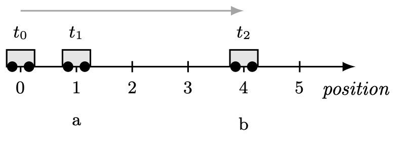
To calculate the speed of the car (i.e., its rate of change of position over time), I would use the following formula:
\[ \text{speed} = \frac{b - a}{t_2 - t_1} \]
This will give the rate of change of position with respect to time.
Now, how can we get the rate of change at a single point in time? For the formula of the rate of change above, we need two distinct points in space (\(a\) and \(b\)) and two distinct points in time. Otherwise, both the numerators and denominators will be \(0\), and \(0/0\) is not a quantity mathematicians like to deal with. More generally, divisions by \(0\) are frowned upon.
Why are divisions by 0 frowned upon?
Imagine the following equality:
\[ \frac{2}{0} = b \]
If division by \(0\) is defined, it would mean that the following equality holds:
\[ 2 = b \cdot 0 \]
I challenge you to find this number \(b\) so that \(b \cdot 0\) equals anything else than \(0\). This note is inspired by Tony Crilly’s 50 Mathematical Ideas, a book I strongly recommend.
Rate of change of a shrinking interval
To avoid the division by \(0\), what if instead of calculating the rate of change at a single point, we calculated the rate of change over a very small interval?
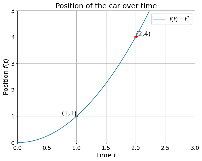
Let’s say that the car has the following position (\(y\)-axis) over time (\(x\)-axis):
Code used to generate the chart
import matplotlib.pyplot as plt
import numpy as np

t = np.linspace(0, 3, 100)
f = t**2

plt.figure(figsize=(8,6))
plt.plot(t, f, label='$f(t) = t^2$')
plt.scatter([1,2], [1,4], color='red')
plt.text(1, 1, '(1,1)', fontsize=16, verticalalignment='bottom', horizontalalignment='right')
plt.text(2, 4, '(2,4)', fontsize=16, verticalalignment='bottom', horizontalalignment='left')
plt.title('Position of the car over time', fontsize=18)
plt.xlabel('Time $t$', fontsize=16)
plt.ylabel('Position $f(t)$', fontsize=16)
plt.xticks(fontsize=14)
plt.yticks(fontsize=14)
plt.xlim(0,3)
plt.ylim(0,5)
plt.legend(fontsize=14)
plt.grid(True)
plt.show()
You can read this chart as: at \(t=1\), the car had a position of \(1\). At \(t=2\) the car had a position of \(4\). More generally, the position of the car at any time \(t\) can be calculated with the function \(f(t) = t^2\).
To check your understanding, what would be the position of the car at \(t=3\)? And \(t=4\)? \(t=256\)? (just kidding, you can skip that last one)
To calculate the rate of change between \(t=1\) and \(t=2\), we can use the formula used above. We get:
\[ \frac{2^2 - 1^2}{2-1} = \frac{4 - 1}{2 - 1} = \frac{3}{1} = 3 \]
The rate of change between these two points is \(3\). Now, what if we pick \(1\) and \(1.5\) instead? We get:
\[ \frac{(1.5)^2 - 1^2}{1.5 - 1} = \frac{2.25 - 1}{0.5} = \frac{1.25}{0.5} = 2.5 \]
Repeating this with \(1\) and \(1.25\), we get:
\[ \frac{(1.25)^2 - 1^2}{1.25 - 1} = \frac{1.5625 - 1}{0.25} = \frac{0.5625}{0.25} = 2.25 \]
Taking an even smaller interval between \(1\) and \(1.1\), we get:
\[ \frac{(1.1)^2 - 1^2}{1.1 - 1} = \frac{1.21 - 1}{0.1} = \frac{0.21}{0.1} = 2.1 \]
You may notice that the smaller the interval, the closer we get to \(2\).
To check your understanding, confirm this last sentence by calculating the rate of change between \(1\) and \(1.01\), and \(1\) and \(1.001\).
\[ \frac{(1.01)^2 - 1^2}{1.01 - 1} = \frac{1.0201 - 1}{0.01} = \frac{0.0201}{0.01} = 2.01 \]
\[ \frac{(1.001)^2 - 1^2}{1.001 - 1} = \frac{1.002001 - 1}{0.001} = \frac{0.002001}{0.001} = 2.001 \]
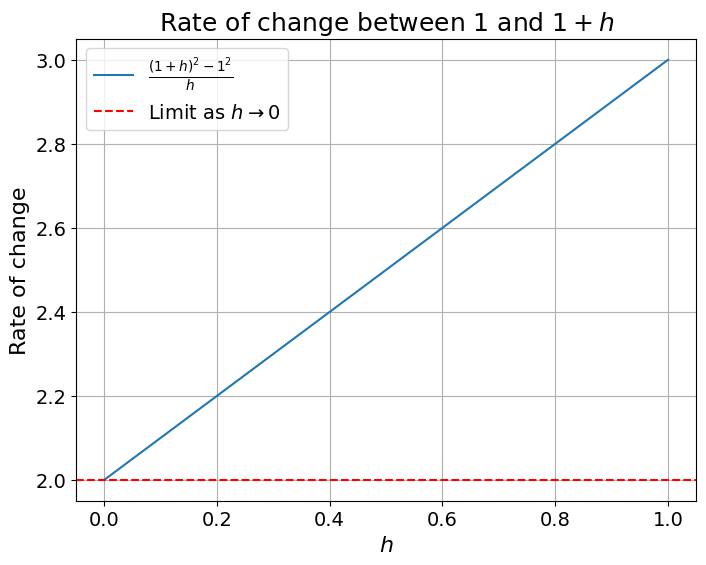
We can confirm this visually by plotting the rate of change between \(1\) and \(1+h\), with \(h\) a positive real number as \(h\) gets closer to \(0\).
Code used to generate the graph
import matplotlib.pyplot as plt
import numpy as np

h = np.linspace(0.001, 1, 100)
rate = ((1 + h)**2 - 1**2) / h

plt.figure(figsize=(8,6))
plt.plot(h, rate, label=r'$\frac{(1+h)^2 - 1^2}{h}$')
plt.axhline(2, color='red', linestyle='--', label='Limit as $h \\to 0$')
plt.title('Rate of change between $1$ and $1+h$', fontsize=18)
plt.xlabel('$h$', fontsize=16)
plt.ylabel('Rate of change', fontsize=16)
plt.xticks(fontsize=14)
plt.yticks(fontsize=14)
plt.legend(fontsize=14)
plt.grid(True)
plt.show()
This graph plots the expression:
\[ \frac{f(1+h) - f(1)}{h} \]
This can be simplified further, expand this if you are interested
\[ \frac{f(1+h) - f(1)}{h} = \frac{(1+h)^2 - 1^2}{h} = \frac{1 + 2h + h^2 - 1}{h} = \frac{2h + h^2}{h} = 2 + h \]
As you can see, this expression converges to \(2\) as \(h\) gets closer and closer to \(0\). As we get closer to \(0\), we get arbitrarily close to the rate of change of the function at a single point (!).
Building the derivative
This is exactly what a derivative is all about. The derivative of a function \(f(x)\) is generally noted \(f'(x)\) and is the rate of change of the function \(f(x)\):
\[ \frac{f(x + h) - f(x)}{h} \]
as the number \(h\) tends towards \(0\). In calculus, this is written:
\[ f'(x) = \lim_{h \to 0} \frac{f(x + h) - f(x)}{h} \]
Using the chart above, we calculated the derivative of \(f(t)\) at \(t=1\). We did so by plotting \(\frac{f(1+h) - f(1)}{h}\) as \(h\) got closer to \(0\) and saw that it converged to \(2\). But do we have a way to know the derivative at any point of this function without all of these plots?
Yes, we do! And we can do this without needing to memorise tens of different rules. Let’s look at the following expression:
\[ \frac{f(x + h) - f(x)}{h} \]
With \(f(x) = x^2\)
We then get:
\[ \frac{f(x + h) - f(x)}{h} = \frac{(x + h)^2 - x^2}{h} \]
\[ = \frac{x^2 + 2x h + h^2 - x^2}{h} \]
\[ = \frac{2x h + h^2}{h} \]
\[ = 2x + h \]
As \(h\) tends towards \(0\), this expression becomes \(2x\), giving us \(f'(x) = 2x\) (!)
With this expression, we can determine the derivative of \(f(x)\) at any \(x\).
To test your understanding, find the derivatives of the following functions:
- \(f(x) = 2 + x\)
- \(f(x) = x^3\)
- \(f(x) = 4x^2\)
Final Thoughts
This was a lot… In this post, we developed a graphical intuition of a derivative as the rate of change of a function at a single point. This paradoxical definition can be made sense of with the concept of limits, something that can be easily visualised. The following post in this series will develop a geometric understanding of derivatives.