The Curse of Dimensionality and its impact on Machine Learning
Imagine entering an abandoned mansion. The front door leads into a room with 10 more doors. Each door you go through will lead you to a similar room with 10 additional doors, with no one or no end in sight.
This could be one way to reason about the curse of dimensionality in Computer Science. There are so many doors, dimensions, and possibilities, that space itself seems to expand.
Dimensionality increases complexity, and this has profound consequences on how we model data.
But what is space? And what are dimensions?
Spaces are generally defined as sets with a particular structure. You can think of a set as a collection: a bag of fruits will be a set. By structure, we mean that space is more than a bag or a set; it has additional properties.
Any point in the space around us has a location, information allowing us to locate it. This location is information along the dimensions of this space. These dimensions are the degrees of freedom, or the directions in which an element can move in that space. In our three-dimensional reality, objects can move along the dimensions of height, width, and depth.
All the items around me right now — my laptop, my notebook, a picture, and my desk lamp — have a location defined by a set of coordinates (“set”, see what I did there?) along the three dimensions of space that I am familiar with. This all refers to only one type of space.
The data we collect about the world can also be represented as points in space. For instance, a population of ducks could be represented on a two-dimensional space of their height and weight, and plotted on a two-dimensional scatter plot:

Code used to generate the plot
import matplotlib.pyplot as plt
import numpy as np
from matplotlib.offsetbox import OffsetImage, AnnotationBbox


np.random.seed(1)
heights = np.random.uniform(15, 50, 15)
weights = np.random.uniform(2, 12, 15)

fig, ax = plt.subplots()

for h, w in zip(heights, weights):
    duck_img = plt.imread("duck.png")
    avg_scale = (h + w*3) / 50
    imagebox = OffsetImage(duck_img, zoom=avg_scale * 0.05)
    ab = AnnotationBbox(imagebox, (w, h), frameon=False)
    ax.add_artist(ab)

ax.set_title("Ducks by Height and Weight", fontsize=18)
ax.set_xlabel("Weight (kg)", fontsize=16)
ax.set_ylabel("Height (cm)", fontsize=16)
ax.tick_params(axis="both", labelsize=14)
ax.set_xlim(0,15)
ax.set_ylim(0,55)
plt.show()
As we collect more information about these ducks such as beak length and width, the number of dimensionality, or the number of dimensions of our data, increases. It becomes impossible to plot these ducks on a web page which only offers two dimensions.
Note: we can also use colours, size of dots, three-dimensional plots, but the human brain is not made to reason over that many dimensions.
History of the concept
The concept of curse of dimensionality was coined by Richard Bellman when working on Dynamic Programming1, a well-known algorithmic paradigm. This problem was originally derived in the context of optimisation.
In optimisation, the more dimensions you add to the space you are searching, the harder it becomes to find an optimum with exhaustive search. As an example, if you are trying to crack a lock with a combination of two digits from 0 to 9 (two finite and discrete dimensions), you can find the time to try all 100 combinations. The number of combinations will increase exponentially with the number of dimensions/digits on the lock, resulting in 10000 combinations for four digits.
This problem also has applications in many other fields such as Machine Learning.
Dimensionality leads to sparsity
As the number of dimensions increases, the total available space increases so fast, that the data available becomes sparse; i.e., few data points in a very large space, or data points very far from one another.
Think of a unit cube, a cube of size one in \(d\) dimensions. Its volume will be \(1^d\) with \(d\) the number of dimensions; which will stay 1, regardless of the number of dimensions.
A cube of size 2 will have volume \(2^d\). In three dimensions, such a cube will have volume \(2^3 = 8\). The difference of size in the unit cube and the cube of size 2 grows exponentially with the number of dimensions. To keep the data density constant, we would need to increase the number of data points exponentially faster than the number of dimensions2.
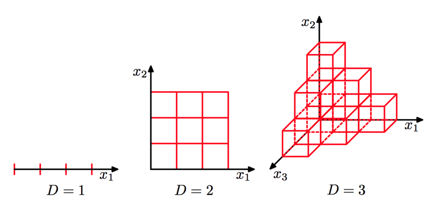 Image credits3
This sparsity can negatively affect many Machine Learning models.
The Consequences of Sparsity
Overfitting
More data dimensions generally means two things for a Machine Learning model:
- more empty space
- more parameters
With more empty space, the model will have space to bend and twist when passing through isolated points.
The number of model parameters tends to increase with the number of features (or dimensions) of the training data. A linear regression with 3 features would generally have 4 parameters: three coefficients and one bias term:
\(y = \beta_0 + \beta_1 x_1 + \beta_2 x_2 + \beta_3 x_3\)
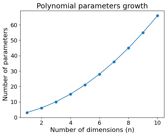
This increase is even more pronounced in polynomial regression of degree \(p\) and \(d\) dimensions:
\(\text{Number of Parameters}=\frac{(p + n)!}{p! \, n!}\)
For a polynomial regression of degree 2 and dimension 3, this would yield 10 parameters; the formula is shown below:
\(f(x_1, x_2, x_3) = \beta_0 + \beta_1 x_1 + \beta_2 x_2 + \beta_3 x_3 + \beta_4 x_1^2 + \beta_5 x_2^2 + \beta_6 x_3^2 + \beta_7 x_1 x_2 + \beta_8 x_1 x_3 + \beta_9 x_2 x_3\)
For example, in 5 dimensions, the number of parameters increases to 21. I will spare you the model equation, but this is how quickly the number of parameters in a degree 2 polynomial increases:
Code used to generate the plot
import matplotlib.pyplot as plt
import numpy as np
from math import comb

degrees = [2]
dimensions = range(1, 11)
params = [comb(d + n, d) for n in dimensions for d in degrees]

fig, ax = plt.subplots()
ax.plot(dimensions, [comb(d + n, d) for n in dimensions for d in degrees], marker='o')

ax.set_title("Polynomial parameters growth", fontsize=18)
ax.set_xlabel("Number of dimensions (n)", fontsize=16)
ax.set_ylabel("Number of parameters", fontsize=16)
ax.tick_params(axis="both", labelsize=14)
plt.show()
This increase of parameters makes models more expressive. This could be an issue when keeping the data size constant and could lead to overfitting. As the model gets more complex, it starts memorising the training data.
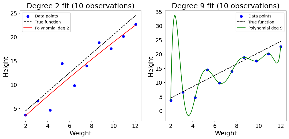
This can be shown with a toy example with 10 random data points, trying to model the height of ducks based on their weight:
Code used to generate the plot
import numpy as np
import matplotlib.pyplot as plt
np.random.seed(2)
# True function for height vs weight
def true_function(x):
return 2*x + 0.5
# Generate 10 data points
weights_10 = np.linspace(2, 12, 10)
heights_10 = true_function(weights_10) + np.random.randn(10)*2
# Fit polynomial of degree 2
coeffs_2 = np.polyfit(weights_10, heights_10, 2)
poly_2 = np.poly1d(coeffs_2)
# Fit polynomial of degree 9
coeffs_9 = np.polyfit(weights_10, heights_10, 9)
poly_9 = np.poly1d(coeffs_9)
# Plot
x_plot = np.linspace(2, 12, 200)
fig, (ax1, ax2) = plt.subplots(1, 2, figsize=(12,5))
ax1.scatter(weights_10, heights_10, c="blue", label="Data points")
ax1.plot(x_plot, true_function(x_plot), 'k--', label="True function")
ax1.plot(x_plot, poly_2(x_plot), 'r-', label="Polynomial deg 2")
ax1.set_title("Degree 2 fit (10 observations)", fontsize=18)
ax1.set_xlabel("Weight", fontsize=16)
ax1.set_ylabel("Height", fontsize=16)
ax1.tick_params(axis="both", labelsize=14)
ax1.legend()
ax2.scatter(weights_10, heights_10, c="blue", label="Data points")
ax2.plot(x_plot, true_function(x_plot), 'k--', label="True function")
ax2.plot(x_plot, poly_9(x_plot), 'g-', label="Polynomial deg 9")
ax2.set_title("Degree 9 fit (10 observations)", fontsize=18)
ax2.set_xlabel("Weight", fontsize=16)
ax2.set_ylabel("Height", fontsize=16)
ax2.tick_params(axis="both", labelsize=14)
ax2.legend()
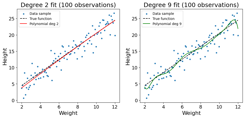
plt.show()As shown in the plot above, the sparsity of the data combined with the high complexity of the polynomial regression of degree 9 leads the model to overfit on the training data. The function twists, bends, and learns the noise of the training data. This problem can somehow be addressed by increasing the number of observations used to 100:
Code used to generate the plot
import numpy as np
import matplotlib.pyplot as plt

np.random.seed(2)

def true_function(x):
    return 2*x + 0.5

# Generate 100 data points
weights = np.linspace(2, 12, 100)
heights = true_function(weights) + np.random.randn(100)*2

# Fit polynomial of degree 2
coeffs_2 = np.polyfit(weights, heights, 2)
poly_2 = np.poly1d(coeffs_2)

# Fit polynomial of degree 9
coeffs_9 = np.polyfit(weights, heights, 9)
poly_9 = np.poly1d(coeffs_9)

# Plot
x_plot = np.linspace(2, 12, 200)
fig, (ax1, ax2) = plt.subplots(1, 2, figsize=(12,5))

ax1.scatter(weights, heights, c="tab:blue", s=10, label="Data sample")
ax1.plot(x_plot, true_function(x_plot), 'k--', label="True function")
ax1.plot(x_plot, poly_2(x_plot), 'r-', label="Polynomial deg 2")
ax1.set_title("Degree 2 fit (100 observations)", fontsize=18)
ax1.set_xlabel("Weight", fontsize=16)
ax1.set_ylabel("Height", fontsize=16)
ax1.tick_params(axis="both", labelsize=14)
ax1.legend()

ax2.scatter(weights, heights, c="tab:blue", s=10, label="Data sample")
ax2.plot(x_plot, true_function(x_plot), 'k--', label="True function")
ax2.plot(x_plot, poly_9(x_plot), 'g-', label="Polynomial deg 9")
ax2.set_title("Degree 9 fit (100 observations)", fontsize=18)
ax2.set_xlabel("Weight", fontsize=16)
ax2.set_ylabel("Height", fontsize=16)
ax2.tick_params(axis="both", labelsize=14)
ax2.legend()

plt.show()
Though still not perfect, we see that the increased data density reduces the likelihood of overfitting. As you may be noticing with the twists of the line at the edges of the dataset, a polynomial regression of degree 9 is still too complex to model such a simple relationship.
Distance metrics become less meaningful
High dimensionality not only leads to overfitting. Some stranger things happen in high dimensions, when distance itself loses its meaning as empty space grows.
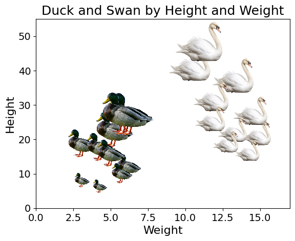
The Nearest Neighbour model in Machine Learning classifies instances based on their proximity with training data points. Let’s imagine a dataset composed of ducks and swans, in a space of two dimensions, height and weight.
Code used to generate the plot
import matplotlib.pyplot as plt
import numpy as np
from matplotlib.offsetbox import OffsetImage, AnnotationBbox

np.random.seed(3)
heights_duck = np.random.uniform(5, 30, 10)
weights_duck = np.random.uniform(3, 8, 10)

heights_swan = np.random.uniform(10, 50, 10)
weights_swan = np.random.uniform(10, 15, 10)

fig, ax = plt.subplots()

# Ducks
for h, w in zip(heights_duck, weights_duck):
    duck_img = plt.imread("duck2.png")
    avg_scale = (h + w) / 300
    imagebox = OffsetImage(duck_img, zoom=avg_scale*0.3)
    ab = AnnotationBbox(imagebox, (w, h), frameon=False)
    ax.add_artist(ab)

# Swans
for h, w in zip(heights_swan, weights_swan):
    swan_img = plt.imread("swan.png")
    avg_scale = (h + w) / 50
    imagebox = OffsetImage(swan_img, zoom=avg_scale*0.2)
    ab = AnnotationBbox(imagebox, (w, h), frameon=False)
    ax.add_artist(ab)

ax.set_title("Duck and Swan by Height and Weight", fontsize=18)
ax.set_xlabel("Weight", fontsize=16)
ax.set_ylabel("Height", fontsize=16)
ax.tick_params(axis="both", labelsize=14)
ax.set_ylim(0,55)
ax.set_xlim(0,17)
plt.show()
When predicting the label (“duck” or “swan”) based on the height and weight of a duck, we find the nearest neighbours of the new data point, and use methods like majority vote. If out of the 5 nearest neighbours of the data point, 3 or more are ducks, we will classify the new bird as a duck. We typically use the Euclidean distance (a generalisation of the Pythagorean theorem) to find the three nearest observations.
Euclidean Distance formula:
\(d(\mathbf{x},\mathbf{y}) = \sqrt{\sum_{i=1}^n (x_i - y_i)^2}\)
This model works in low-dimensional space as the Euclidean distance still makes sense. Strange things start happening in high dimensions. As the space grows exponentially, data points become further and further apart, and the notion of “nearest neighbour” becomes inappropriate.
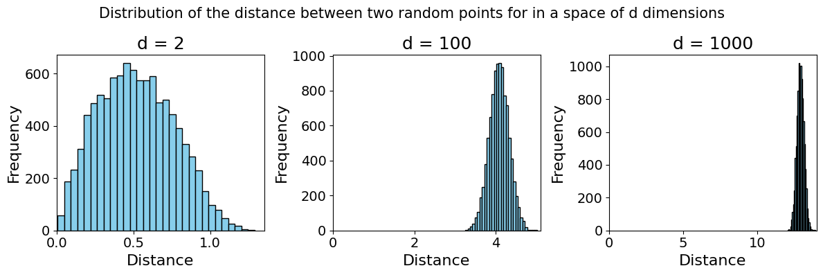
See below an example of two independent variables \(X\) and \(Y\) (representing randomly sampled points) in a space of \([0,1]^d\), a space of \(d\) continuous dimensions, each going from 0 to 1. Over 100 trials of sampling both points and calculating the distance between the two, we observe that they grow further and further apart4
Code used to generate the plot
import numpy as np
import matplotlib.pyplot as plt

def average_distance(d, n=100, trials=100):
    distances = []
    for _ in range(trials):
        x = np.random.rand(n, d)
        y = np.random.rand(n, d)
        # Euclidean distance between x and y in d-dim
        dist = np.sqrt(np.sum((x - y)**2, axis=1))
        distances.append(np.mean(dist))
    return np.mean(distances)

dims = [2, 100, 1000]
avg_dists = [average_distance(d) for d in dims]

fig, axes = plt.subplots(1, 3, figsize=(12, 4))
for ax, d, dist in zip(axes, dims, avg_dists):
    ax.bar(str(d), dist, color="skyblue")
    ax.set_title(f"d = {d}", fontsize=18)
    ax.tick_params(axis="both", labelsize=14)
    ax.set_ylim(0, max(avg_dists)*1.1)
    ax.set_ylabel("Average Distance", fontsize=16)
plt.tight_layout()
plt.show()
Example of high-dimensional ML problems
Representing the weight and height of birds is a simple problem. Many Machine Learning problems involve much higher-dimensional data, examples include:
- Images: a small black and white image of 100×100 pixels would already have 10000 parameters. If the image has colours, each pixel would have three channels, tripling the number of parameters.
Text: a single word can be viewed as a vector of the dimension of the vocabulary size, filled with 0s, with a single 1 at the index of the word.
Consider a vocabulary containing only four words: [“duck”, “goose”, “swan”, “hen”]. There, each word could be represented in four dimensions. “duck” would be represented as the vector: [1,0,0,0], and “swan” [0,0,1,0]. To apply this to the English language, we would need vectors with size of around 50,000 to represent a single word. A document of 100 words would then have a dimensionality of 100 × 50,000.Genomic data: the human genome is composed of more than 3 billion base pairs (the duck genome is approximately 1.26 billion), only thinking about modelling such a high dimensionality hurts.
Practical recommendations
This section will stray away from theoretical ideas into Machine Learning applications. If you are not interested in these, head directly to the conclusion.
Feature engineering and selection
Looking at the impact of the curse of dimensionality on Machine Learning models, it is a good idea to wisely select the features of the training data. They define the space in which the data will be represented. There are many different ways to select features, which could be the subject of another blog post entirely. My recommendation would be to explore the following high-level categories:
Common sense
Include the information you think the model would benefit from.Filter-based methods
You can use correlation between features or between features and the target variables to eliminate less informative features.Feature importance
Check the feature importance of all features and experiment with removing unimportant features. While applying this method, one must remember that feature importance asks the question: what is the importance of this feature on my model trained on a given set of features? It cannot tell you the importance a feature would have had using another feature set.Feature Engineering as an optimisation problem
This last method views feature engineering as an optimisation problem, with a decision variable per feature (“use” or “not use”). The idea is to experiment retraining a model with different feature sets and selecting the one generating the best model performance. To make this computationally feasible, I would recommend using multi-fidelity optimisation.
Regularisation
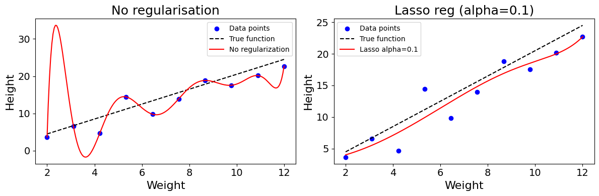
Regularisation methods can be used to constrain model complexity regardless of the number of parameters and dimensions. In the example of the polynomial models above, we could include a regularisation parameter to the loss function, to constrain the value of the regression coefficient. This will smoothen the model and prevent it from twisting.
The equation below shows what a loss function with Lasso constraint looks like. The model is penalised for higher parameter values.
\(L(\beta) = \sum_{i=1}^{n} (y_i - \hat{y_i})^2 + \lambda \sum_{j=1}^{d} |\beta_j|\)
Note: when modelling, we generally specify the \(\alpha\) parameter, with \(\lambda = \frac{1}{\alpha}\). The smaller the \(\alpha\), the stronger the regularisation.
Code used to generate the plot
import numpy as np
import matplotlib.pyplot as plt
from sklearn.linear_model import Lasso, LinearRegression
np.random.seed(2)

def true_function(x):
    return 2*x + 0.5

weights_small = np.linspace(2, 12, 10)
heights_small = true_function(weights_small) + np.random.randn(10)*2

x_plot = np.linspace(2, 12, 200)
fig, (ax1, ax2) = plt.subplots(1, 2, figsize=(12, 4))

# No regularization
poly_features = np.column_stack([weights_small**i for i in range(0,10)])
model = LinearRegression().fit(poly_features, heights_small)

poly_plot = np.column_stack([x_plot**i for i in range(0,10)])
y_plot = model.predict(poly_plot)

ax1.scatter(weights_small, heights_small, c="blue", label="Data points")
ax1.plot(x_plot, true_function(x_plot), 'k--', label="True function")
ax1.plot(x_plot, y_plot, 'r-', label="No regularization")
ax1.set_title("No regularisation", fontsize=18)
ax1.set_xlabel("Weight", fontsize=16)
ax1.set_ylabel("Height", fontsize=16)
ax1.tick_params(axis="both", labelsize=14)
ax1.legend()

# Lasso with alpha=0.1
model = Lasso(alpha=0.1, max_iter=100000).fit(poly_features, heights_small)
y_plot = model.predict(poly_plot)

ax2.scatter(weights_small, heights_small, c="blue", label="Data points")
ax2.plot(x_plot, true_function(x_plot), 'k--', label="True function")
ax2.plot(x_plot, y_plot, 'r-', label="Lasso alpha=0.1")
ax2.set_title("Lasso reg (alpha=0.1)", fontsize=18)
ax2.set_xlabel("Weight", fontsize=16)
ax2.set_ylabel("Height", fontsize=16)
ax2.tick_params(axis="both", labelsize=14)
ax2.legend()

plt.tight_layout()
plt.show()
Dimensionality reduction
There are many different methods to reduce the dimensionality of a dataset. A technique like Principal Component Analysis (PCA) aims to isolate the components, linear combinations of features, that account for the largest share of the variance in the dataset.
PCA is one of many manifold learning techniques which aim to project high-dimensional data into a lower-dimensional space. Other frequently-used non-linear methods include t-SNE or UMAP.
Large Language Models (LLMs), such as Transformers and Encoders, allow us to reduce the dimensionality of text-based data through embeddings. Through this process, words and documents can be projected into a continuous set of finite dimensions. In other words, a word, sentence, or entire document could be converted to a vector of numbers.
Built-in model Regularisation
Many model types include some kind of embedded regularisation. Convolutional Neural Networks use weight-sharing to deal with the high dimensionality of image inputs. Thanks to this sharing, the number of parameters does not grow exponentially with the dimensionality of the image.
Neural Networks can also be trained with dropout, randomly deactivating a subset of neurons in the computational graph at each training iteration. Additional constraints can also be applied to weights during training (“weight decay”) to prevent the model from overfitting on the training data.
Final Thoughts
“The more he analyzes the universe into infinitesimals, the things he finds to classify, and the more he perceives the relativity of all classification. What he does not know seems to increase in geometric progression to what he knows.” The Wisdom of Insecurity, Alan Watts
The more dimensions we add, or the higher the dimensionality of the space we explore, the less we know, and the sparser our data becomes. The curse of dimensionality is one of the most fascinating problems in Computer Science. It is by building algorithms that can overcome this challenge that we start modelling the complexity of our world.
Footnotes
R. Bellman, Adaptive Control Processes: A Guided Tour. Princeton, NJ, USA: Princeton University Press, 1961.↩︎
R. Vershynin, High-Dimensional Probability and Applications in Data Science. Retrieved from https://www.math.uci.edu/~rvershyn/teaching/hdp/hdp.html, Chapter 1.↩︎
J. Delon, The Curse of Dimensionality. Retrieved from https://mathematical-coffees.github.io/slides/mc08-delon.pdf.↩︎
J. Delon, The Curse of Dimensionality. Retrieved from https://mathematical-coffees.github.io/slides/mc08-delon.pdf.↩︎