What SHAP values actually are and how to compute them
Have you ever seen one of these plots?
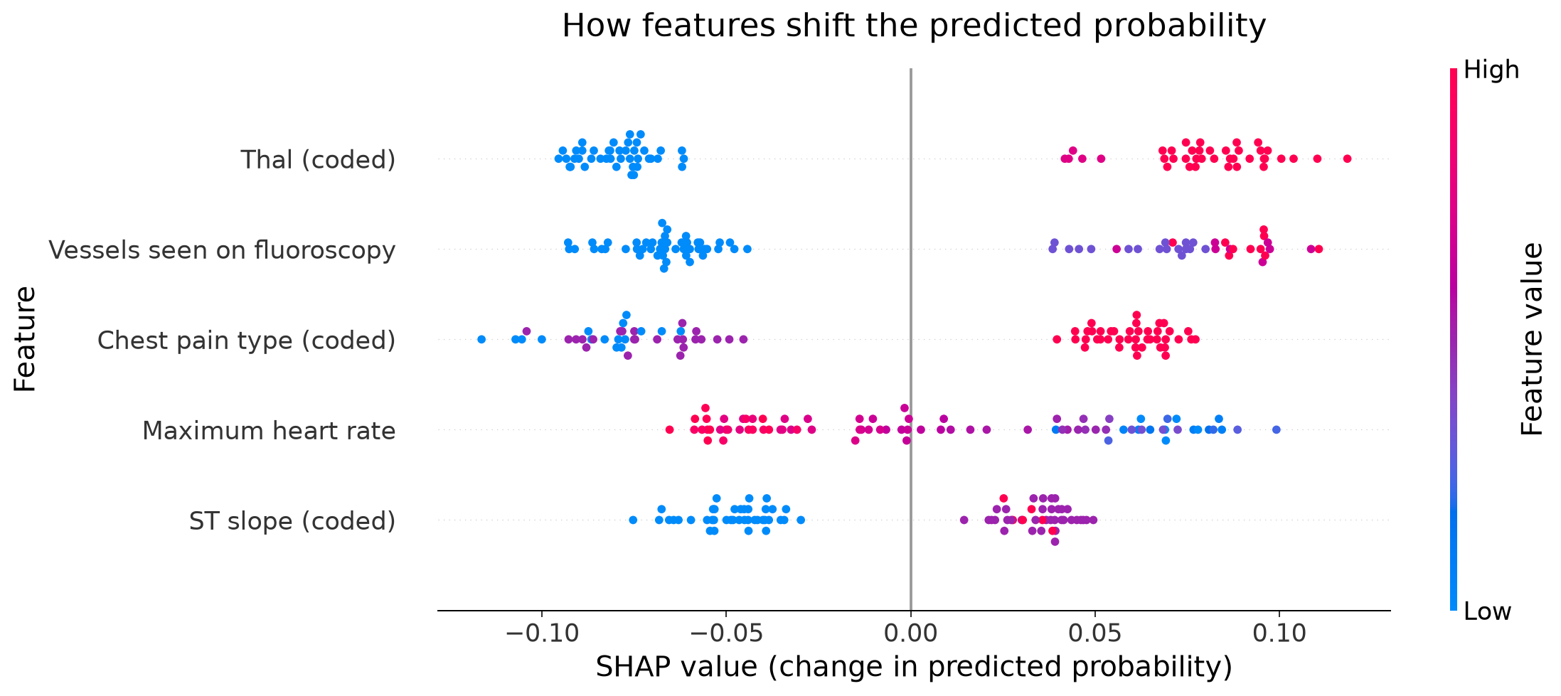
How would you explain what the dots are, or how they are calculated?
Another common plot is the waterfall plot, which explains a single prediction:
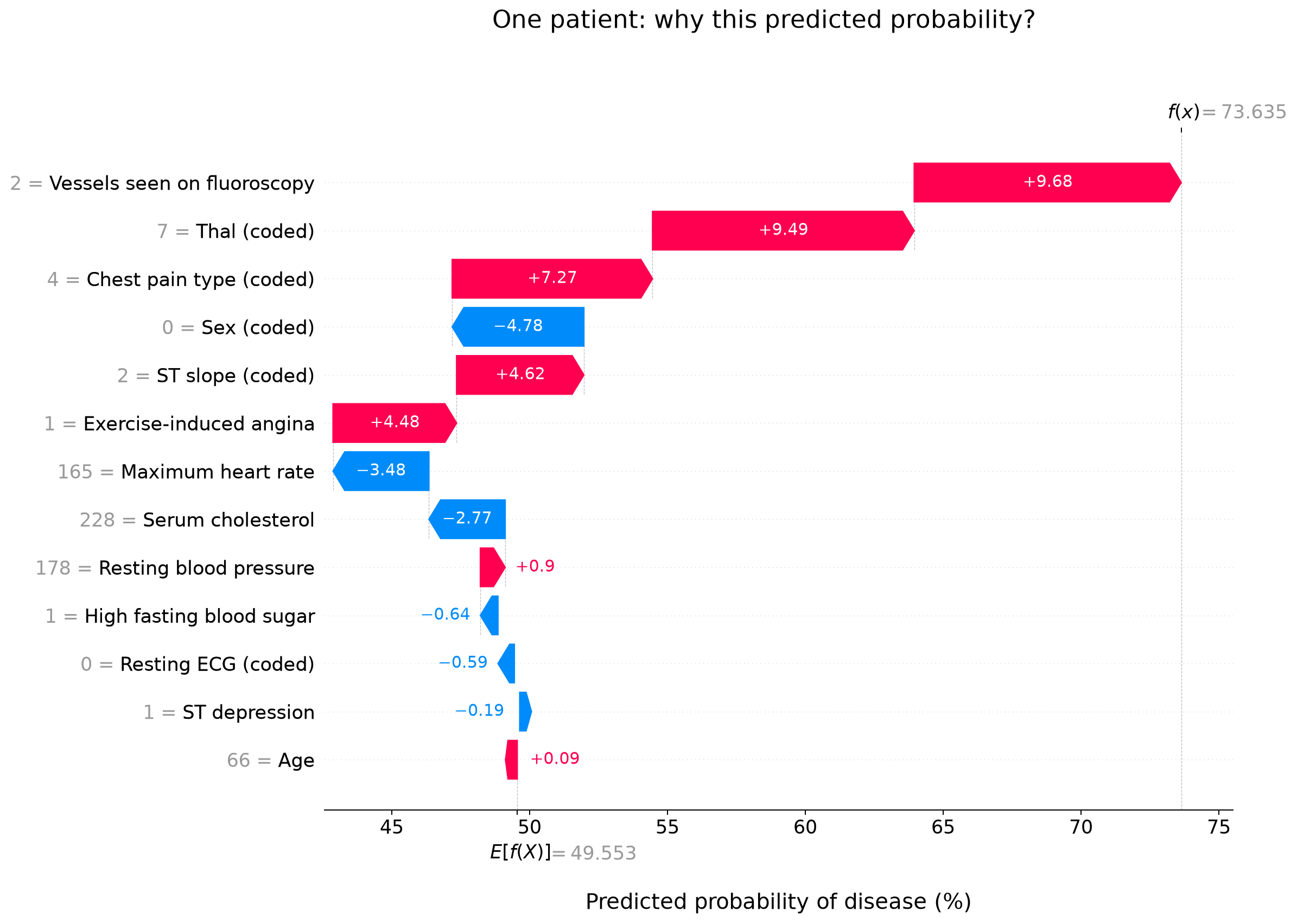
The beeswarm plot above collects these individual contributions across patients: each dot is one patient’s contribution for one feature. But how do we calculate those contributions in the first place?
Before writing this article, I could not. I also found it surprisingly difficult to learn without getting lost in mathematical jargon. By the end of this post, you should get an intuitive understanding of SHAP values and have an idea of how to compute them if the shap package were to disappear tomorrow.
When asking machine learning professionals about SHAP values (I tried this with my friends), they would tell me: “It is a game-theoretical approach to measure feature importance, blah, blah, blah…”. Keep asking, though, and the explanation will quickly dry up.
This is the big paradox with SHAP values: everyone uses them for interpretability, and so few people understand how they are calculated. The underlying maths is really not bad.
The Intuition
To make this chapter more concrete, we will use the Statlog Heart dataset, predicting the presence of heart disease using medical observations. It contains 270 patients and 13 features. We use a Random Forecast model to predict this binary outcome.
In a machine learning context, SHAP values answer the question: what is the contribution of this single feature value to this prediction?
For instance, what was the impact of this patient having two major vessels visible on fluoroscopy (feature value) on the predicted probability of disease (prediction)?
In other words, had the feature value not been there, what would have been the change in the final prediction? SHAP makes this precise by averaging the change across different combinations of other known feature values. This explains the model’s prediction, rather than establishing a medical cause.
Putting this into maths
Let’s put this in a slightly more rigorous form.
For observation \(x\), the contribution of feature \(i\) in one context is the prediction with its value known minus the prediction with its value unknown:
\[ \Delta_i(S; x) = v_x(S \cup \{i\}) - v_x(S). \]
With:
- \(F\) the set of all feature indices, for example \(F = \{1, 2, 3\}\) for age, blood pressure and cholesterol
- \(S\) a subset of those indices, for example \(S = \{1, 3\}\), with \(i \notin S\)
- \(v_x(S)\) the average prediction when we keep the values of \(x\) for features in \(S\) and replace the remaining values using a background dataset
The SHAP value is the weighted average contribution from adding feature \(i\) to all possible subsets \(S\) that do not contain \(i\).
Taking the formula part by part:
- \(v_x(S \cup \{i\})\) is the average prediction after adding the observed value of feature \(i\) to subset \(S\)
- \(v_x(S)\) is the average prediction with only the observed values for \(S\) retained
For example, with \(S = \{1, 3\}\) and \(i = 2\), the marginal contribution of blood pressure is:
\[ \Delta_2(\{1, 3\}; x) = v_x(\{1, 2, 3\}) - v_x(\{1, 3\}). \]
If these two predictions are \(0.70\) and \(0.55\), the marginal contribution is \(0.15\), or 15 percentage points. This is one contribution to average, not yet the SHAP value.
If I know this quantity over all possible subsets and apply the appropriate weights, I have the answer to the original question:
Had the feature value not been there, what would have been the change in the final prediction, averaged over those contexts?
What does it mean for a feature not to be there?
This is one of the trickiest aspects of SHAP value calculations. We cannot really “remove” a feature from a model. The machine learning model was already trained.
One way to do so is to replace a given feature value with other values of this feature in a background sample from the training set, then generate predictions with the trained model for each of these replacements.
The average of these predictions estimates what the prediction would be when we do not know that feature value. When several features are missing, we take their replacement values together from each background row.
Let’s use a simple linear model with three features:
\[ f(x) = 2 \cdot x_1 + 3 \cdot x_2 + x_3. \]
Here are ten example rows and their predictions:
| Row | \(x_1\) | \(x_2\) | \(x_3\) | \(f(x)\) |
|---|---|---|---|---|
| 1 | 4 | 2 | 3 | 17 |
| 2 | 1 | 1 | 2 | 7 |
| 3 | 2 | 3 | 1 | 14 |
| 4 | 3 | 2 | 4 | 16 |
| 5 | 5 | 1 | 2 | 15 |
| 6 | 2 | 4 | 3 | 19 |
| 7 | 1 | 2 | 5 | 13 |
| 8 | 4 | 3 | 2 | 19 |
| 9 | 3 | 4 | 1 | 19 |
| 10 | 5 | 2 | 4 | 20 |
Imagine we want to compute the SHAP value for feature \(1\) at row \(1\). We can write this row as a dictionary of feature values:
\[ x = \{\text{feature } 1: 4,\quad \text{feature } 2: 2,\quad \text{feature } 3: 3\}. \]
First, consider the subset containing only feature \(3\):
\[ S = \{3\}. \]
We need to pretend that features \(1\) and \(2\) are unknown. This is where sampling comes in. Suppose our background sample consists of these three other training rows (more would usually be needed in practice):
| Row | \(x_1\) | \(x_2\) | \(x_3\) | \(f(x)\) |
|---|---|---|---|---|
| 2 | 1 | 1 | 2 | 7 |
| 3 | 2 | 3 | 1 | 14 |
| 4 | 3 | 2 | 4 | 16 |
These are our background rows, training examples that supply replacement values for the features we pretend not to know. For each background row, we keep the feature values in \(S\) from the observation we are explaining, replace the remaining values with those from that background row, and make a prediction.
We then take an average of these predictions to obtain \(v_x(S)\).
To get \(v_x(\{3\})\), keep \(x_3 = 3\) and average over the three replacements for features \(1\) and \(2\):
\[ \begin{aligned} v_x(\{3\}) &= \frac{1}{3} \cdot \bigl(f(1, 1, 3) + f(2, 3, 3) + f(3, 2, 3)\bigr) \\ &= \frac{1}{3} \cdot (8 + 16 + 15) = 13. \end{aligned} \]
After adding feature \(1\), we keep both \(x_1 = 4\) and \(x_3 = 3\):
\[ \begin{aligned} v_x(\{1, 3\}) &= \frac{1}{3} \cdot \bigl(f(4, 1, 3) + f(4, 3, 3) + f(4, 2, 3)\bigr) \\ &= \frac{1}{3} \cdot (14 + 20 + 17) = 17. \end{aligned} \]
The marginal contribution is therefore:
\[ \Delta_1(\{3\}; x) = 17 - 13 = 4. \]
SHAP value calculation
There is one more trick in the calculation of SHAP values: not all feature subsets receive the same individual weight.
Two useful contexts for understanding the contribution of a single feature are:
- The empty subset \(\varnothing\)
- The full set of other features \(F \setminus \{i\}\)
Why?
When adding a feature to the empty subset, you measure its contribution when no other feature values are known:
\[ v_x(\{i\}) - v_x(\varnothing). \]
The empty-subset value is the average model prediction over the background rows. Writing \(B\) for the number of background rows and \(b^{(r)}\) for row \(r\):
\[ v_x(\varnothing) = \frac{1}{B} \cdot \sum_{r=1}^{B} f(b^{(r)}). \]
On the other hand, the full set of other features tells you what happens when you remove a given feature value from the full input:
\[ v_x(F) - v_x(F \setminus \{i\}). \]
This section will describe the weight function in further details. You do not need to memorise this formula. It is only important to remember that the empty subset and the nearly full subset receive the largetst individual weights.
For \(m = |F|\) features, the weight function is the following (big formula warning):
\[ w(S) = \frac{|S|! \cdot (m - |S| - 1)!}{m!}. \]
There are \(|S|!\) ways to order the features before \(i\) and \((m - |S| - 1)!\) ways to order those after it, out of \(m!\) total orders.
This is very, very scary. Before we get into it, we can visualise this weight for a dataset of ten features, \(|F| = 10\):
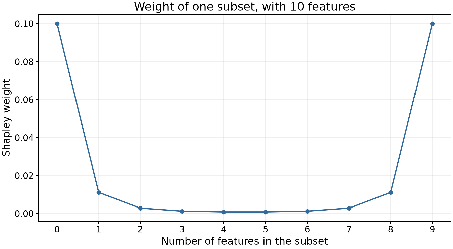
This already looks a lot more familiar. It is a symmetric U-shaped curve that assigns a higher value to each empty or nearly full subset.
The weight is also the inverse of a binomial coefficient, divided by the number of features:
\[ w(S) = \frac{1}{m \cdot \binom{m - 1}{|S|}}. \]
There are \(\binom{m - 1}{s}\) subsets of size \(s\), so their total weight is always \(1/m\). Small and large subsets receive larger individual weights because there are fewer of them, rather than because their sizes deserve more total influence.
Counting combinations with binomial coefficients
The notation \(\binom{n}{k}\), also written \({}_nC_k\), is the number of ways you can pick \(k\) items out of \(n\) items when the order does not matter. Putting numbers into the formula, \(\binom{3}{2}\) is the number of ways in which you can pick two items out of three items.
Imagine you have three objects: a tomato, an apple and an orange. There are three ways you can pick two items:
- Tomato and apple
- Apple and orange
- Tomato and orange
With three items, this is very easy to compute. But what would \(\binom{10}{3}\) be?
To compute this, we can use the general formula:
\[ \binom{n}{k} = \frac{n!}{k! \cdot (n-k)!}. \]
The expression \(n!\) is read “ \(n\) factorial” and, for a positive integer \(n\), is defined as:
\[ n! = n \cdot (n-1) \cdot \ldots \cdot 2 \cdot 1. \]
For example, \(3! = 3 \cdot 2 \cdot 1 = 6\) and \(0! = 1\) (this last one is confusing, the topic of another article).
This gives:
\[ \binom{10}{3} = \frac{10 \cdot 9 \cdot 8}{3 \cdot 2 \cdot 1} = 120. \]
To make sure you understand this concept, compute \(\binom{2}{1}\), \(\binom{4}{3}\) and \(\binom{4}{4}\).
Putting it all together
With all the elements seen above, we can compute SHAP values. We note the SHAP value of feature \(i\) as \(\phi_i(x)\). We have to compute the following weighted average:
\[ \phi_i(x) = \sum_{S \subseteq F \setminus \{i\}} \frac{|S|! \cdot (m - |S| - 1)!}{m!} \cdot \bigl[v_x(S \cup \{i\}) - v_x(S)\bigr]. \]
The weights give each subset size the same total influence. The empty subset and the full set without feature \(i\) each receive weight \(1/m\).
Compute exact SHAP values in Python
This small implementation enumerates every subset, using NumPy and the Python standard library. It works with a prediction function that returns one number per row.
from itertools import combinations
from math import comb
import numpy as np


def exact_shap(predict, x, background):
    m = len(x)
    values = {}
    for size in range(m + 1):
        for subset in combinations(range(m), size):
            hybrid = background.copy()
            hybrid[:, list(subset)] = x[list(subset)]
            values[frozenset(subset)] = predict(hybrid).mean()

    phi = np.zeros(m)
    for i in range(m):
        for subset, value in values.items():
            if i not in subset:
                weight = 1 / (m * comb(m - 1, len(subset)))
                phi[i] += weight * (values[subset | {i}] - value)
    return phi


x = np.array([4., 2., 3.])
background = np.array([[1., 1., 2.], [2., 3., 1.], [3., 2., 4.]])
predict = lambda rows: rows @ np.array([2., 3., 1.])
print(exact_shap(predict, x, background))
# [4.         0.         0.66666667]
Once we have these, we can build the charts like the beeswarm plot that we are all familiar with:
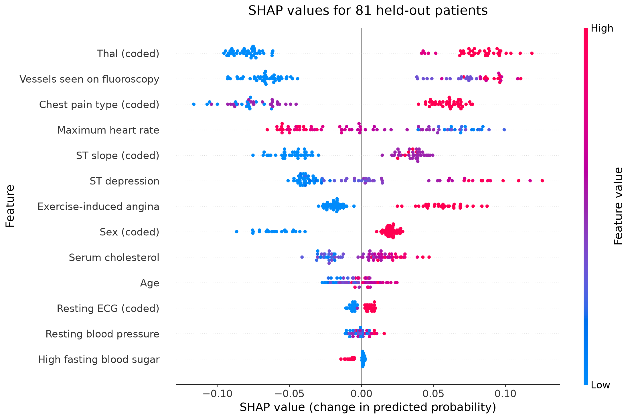
Each dot here is a SHAP value for a given feature and a given sample. Its horizontal position shows whether the contribution is negative or positive, and by how much. Its colour shows the original feature value, from low (blue) to high (red), as in the SHAP beeswarm documentation.
Are we already done?
Well, not really. For a dataset of 1,000 rows and 100 features, how many predictions would you need to generate to compute the following for every feature and row?
\[ \phi_i(x) = \sum_{S \subseteq F \setminus \{i\}} w(S) \cdot \bigl[v_x(S \cup \{i\}) - v_x(S)\bigr]. \]
For each evaluation, we need to fill in the values of features that are not in the subset. We do not need to retrain the model. We do need to compute predictions using \(B = 20\) background rows, for example, as explained in the section on missing features.
For each of the \(100{,}000\) SHAP values (feature and row combinations), there are \(2^{99}\) subsets of the other 99 features. Each marginal contribution involves two subset evaluations. A naive calculation without reusing any evaluations would therefore require:
\[ 1{,}000 \cdot 100 \cdot 2^{99} \cdot 2 \cdot 20 \approx 2.54 \cdot 10^{36} \]
individual input-row predictions.
This is crazy.
For this reason, there is a range of methods that estimate SHAP values without exhaustively calculating the weighted sum:
\[ \sum_{S \subseteq F \setminus \{i\}} w(S) \cdot \bigl[v_x(S \cup \{i\}) - v_x(S)\bigr]. \]
For tree models, specialised algorithms such as TreeSHAP can avoid this exhaustive enumeration. Our plots use KernelSHAP, which also works with general models.
Estimating SHAP values with KernelSHAP
How would this work?
You would sample subsets \(S\) and compute \(v_x(S)\) for each. You then fit a weighted linear regression to learn how subset membership maps to \(v_x(S)\), for one fixed observation \(x\).
Represent the subset by a binary vector \(z\), where \(z_j = 1\) if \(j \in S\) and \(z_j = 0\) otherwise:
For example, with ten features, keeping only features \(1\) and \(3\) gives:
\[ S = \{1, 3\} \quad \longrightarrow \quad z = (1, 0, 1, 0, 0, 0, 0, 0, 0, 0). \]
The first and third entries are \(1\) because those feature values are retained. Every other entry is \(0\) because its value is replaced using the background rows. The regression then maps this vector to the subset’s average prediction:
\[ S \longrightarrow z \longrightarrow g(z) = \phi_0 + \sum_{j=1}^{m} \phi_j \cdot z_j \approx v_x(S). \]
Let’s make this a bit more visual with an invented ten-feature dataset. To keep the arithmetic easy to check, use the linear model:
\[ \begin{aligned} f(x) ={}& 0.1 \cdot x_1 + 0.2 \cdot x_2 + 0.3 \cdot x_3 + 0.4 \cdot x_4 + 0.5 \cdot x_5 \\ &+ 0.6 \cdot x_6 + 0.7 \cdot x_7 + 0.8 \cdot x_8 + 0.9 \cdot x_9 + 1.0 \cdot x_{10}. \end{aligned} \]
Here are its ten rows and their predictions:
| Row | \(x_{1}\) | \(x_{2}\) | \(x_{3}\) | \(x_{4}\) | \(x_{5}\) | \(x_{6}\) | \(x_{7}\) | \(x_{8}\) | \(x_{9}\) | \(x_{10}\) | \(f(x)\) |
|---|---|---|---|---|---|---|---|---|---|---|---|
| 1 | 0 | 4 | 3 | 2 | 2 | 5 | 0 | 4 | 1 | 0 | 10.60 |
| 2 | 3 | 5 | 4 | 4 | 4 | 4 | 3 | 0 | 5 | 2 | 17.10 |
| 3 | 3 | 2 | 1 | 5 | 4 | 3 | 2 | 4 | 3 | 2 | 16.10 |
| 4 | 2 | 1 | 0 | 3 | 5 | 0 | 5 | 4 | 1 | 3 | 14.70 |
| 5 | 0 | 4 | 4 | 2 | 0 | 5 | 2 | 5 | 4 | 4 | 18.80 |
| 6 | 4 | 1 | 2 | 2 | 2 | 0 | 3 | 0 | 4 | 4 | 12.70 |
| 7 | 5 | 4 | 2 | 5 | 2 | 1 | 5 | 2 | 0 | 2 | 12.60 |
| 8 | 4 | 1 | 2 | 0 | 4 | 2 | 1 | 1 | 3 | 4 | 12.60 |
| 9 | 5 | 2 | 0 | 4 | 3 | 4 | 0 | 1 | 4 | 4 | 14.80 |
| 10 | 2 | 4 | 5 | 2 | 5 | 1 | 1 | 4 | 3 | 0 | 13.00 |
We will explain row \(1\), using all ten rows as the fixed background. For this dataset, I could select a few subsets of different sizes:
\[ \varnothing,\quad \{1, 2, 3\},\quad \{4, 5, 6\},\quad \{1, 3\},\quad \{2, 5, 7, 9\},\quad \{2, 3, \ldots, 10\},\quad F. \]
Compute \(v_x(S)\) for each of these subsets (as we did in the previous section). The results are in the following table:
| \(S\) | \(v_x(S)\) |
|---|---|
| \(\varnothing\) | 14.30 |
| \(\{1, 2, 3\}\) | 14.47 |
| \(\{4, 5, 6\}\) | 14.89 |
| \(\{1, 3\}\) | 14.23 |
| \(\{2, 5, 7, 9\}\) | 10.83 |
| \(\{2, 3, 4, 5, 6, 7, 8, 9, 10\}\) | 10.88 |
| \(\{1, 2, 3, 4, 5, 6, 7, 8, 9, 10\}\) | 10.60 |
For example, retaining features \(1\) and \(3\) gives:
\[ v_x(\{1, 3\}) = \frac{1}{10} \cdot x_1 + \frac{3}{10} \cdot x_3 + \sum_{j \notin \{1, 3\}} \frac{j}{10} \cdot \overline{b}_j, \]
where \(\overline{b}_j\) is the background mean of feature \(j\).
Run a weighted linear regression over these evaluations, with the following dataset. Each row is a subset; the binary columns indicate which values are retained, and the target is \(v_x(S)\). We add all single-feature subsets and all subsets missing one feature so there is enough information to identify the coefficients. The preview below shows the same seven subsets as above; expand the note to see all 26 subsets:
| \(S\) | \(z_{1}\) | \(z_{2}\) | \(z_{3}\) | \(z_{4}\) | \(z_{5}\) | \(z_{6}\) | \(z_{7}\) | \(z_{8}\) | \(z_{9}\) | \(z_{10}\) | \(v_x(S)\) |
|---|---|---|---|---|---|---|---|---|---|---|---|
| \(\varnothing\) | 0 | 0 | 0 | 0 | 0 | 0 | 0 | 0 | 0 | 0 | 14.30 |
| \(\{1, 2, 3\}\) | 1 | 1 | 1 | 0 | 0 | 0 | 0 | 0 | 0 | 0 | 14.47 |
| \(\{4, 5, 6\}\) | 0 | 0 | 0 | 1 | 1 | 1 | 0 | 0 | 0 | 0 | 14.89 |
| \(\{1, 3\}\) | 1 | 0 | 1 | 0 | 0 | 0 | 0 | 0 | 0 | 0 | 14.23 |
| \(\{2, 5, 7, 9\}\) | 0 | 1 | 0 | 0 | 1 | 0 | 1 | 0 | 1 | 0 | 10.83 |
| \(\{2, 3, 4, 5, 6, 7, 8, 9, 10\}\) | 0 | 1 | 1 | 1 | 1 | 1 | 1 | 1 | 1 | 1 | 10.88 |
| \(\{1, 2, 3, 4, 5, 6, 7, 8, 9, 10\}\) | 1 | 1 | 1 | 1 | 1 | 1 | 1 | 1 | 1 | 1 | 10.60 |
| \(\vdots\) | \(\vdots\) | \(\vdots\) | \(\vdots\) | \(\vdots\) | \(\vdots\) | \(\vdots\) | \(\vdots\) | \(\vdots\) | \(\vdots\) | \(\vdots\) | \(\vdots\) |
Full dataset used for the weighted regression
| \(S\) | \(z_{1}\) | \(z_{2}\) | \(z_{3}\) | \(z_{4}\) | \(z_{5}\) | \(z_{6}\) | \(z_{7}\) | \(z_{8}\) | \(z_{9}\) | \(z_{10}\) | \(v_x(S)\) |
|---|---|---|---|---|---|---|---|---|---|---|---|
| \(\varnothing\) | 0 | 0 | 0 | 0 | 0 | 0 | 0 | 0 | 0 | 0 | 14.30 |
| \(\{1, 2, 3\}\) | 1 | 1 | 1 | 0 | 0 | 0 | 0 | 0 | 0 | 0 | 14.47 |
| \(\{4, 5, 6\}\) | 0 | 0 | 0 | 1 | 1 | 1 | 0 | 0 | 0 | 0 | 14.89 |
| \(\{1, 3\}\) | 1 | 0 | 1 | 0 | 0 | 0 | 0 | 0 | 0 | 0 | 14.23 |
| \(\{2, 5, 7, 9\}\) | 0 | 1 | 0 | 0 | 1 | 0 | 1 | 0 | 1 | 0 | 10.83 |
| \(\{2, 3, 4, 5, 6, 7, 8, 9, 10\}\) | 0 | 1 | 1 | 1 | 1 | 1 | 1 | 1 | 1 | 1 | 10.88 |
| \(\{1, 2, 3, 4, 5, 6, 7, 8, 9, 10\}\) | 1 | 1 | 1 | 1 | 1 | 1 | 1 | 1 | 1 | 1 | 10.60 |
| \(\{1\}\) | 1 | 0 | 0 | 0 | 0 | 0 | 0 | 0 | 0 | 0 | 14.02 |
| \(\{2\}\) | 0 | 1 | 0 | 0 | 0 | 0 | 0 | 0 | 0 | 0 | 14.54 |
| \(\{3\}\) | 0 | 0 | 1 | 0 | 0 | 0 | 0 | 0 | 0 | 0 | 14.51 |
| \(\{4\}\) | 0 | 0 | 0 | 1 | 0 | 0 | 0 | 0 | 0 | 0 | 13.94 |
| \(\{5\}\) | 0 | 0 | 0 | 0 | 1 | 0 | 0 | 0 | 0 | 0 | 13.75 |
| \(\{6\}\) | 0 | 0 | 0 | 0 | 0 | 1 | 0 | 0 | 0 | 0 | 15.80 |
| \(\{7\}\) | 0 | 0 | 0 | 0 | 0 | 0 | 1 | 0 | 0 | 0 | 12.76 |
| \(\{8\}\) | 0 | 0 | 0 | 0 | 0 | 0 | 0 | 1 | 0 | 0 | 15.50 |
| \(\{9\}\) | 0 | 0 | 0 | 0 | 0 | 0 | 0 | 0 | 1 | 0 | 12.68 |
| \(\{10\}\) | 0 | 0 | 0 | 0 | 0 | 0 | 0 | 0 | 0 | 1 | 11.80 |
| \(\{1, 3, 4, 5, 6, 7, 8, 9, 10\}\) | 1 | 0 | 1 | 1 | 1 | 1 | 1 | 1 | 1 | 1 | 10.36 |
| \(\{1, 2, 4, 5, 6, 7, 8, 9, 10\}\) | 1 | 1 | 0 | 1 | 1 | 1 | 1 | 1 | 1 | 1 | 10.39 |
| \(\{1, 2, 3, 5, 6, 7, 8, 9, 10\}\) | 1 | 1 | 1 | 0 | 1 | 1 | 1 | 1 | 1 | 1 | 10.96 |
| \(\{1, 2, 3, 4, 6, 7, 8, 9, 10\}\) | 1 | 1 | 1 | 1 | 0 | 1 | 1 | 1 | 1 | 1 | 11.15 |
| \(\{1, 2, 3, 4, 5, 7, 8, 9, 10\}\) | 1 | 1 | 1 | 1 | 1 | 0 | 1 | 1 | 1 | 1 | 9.10 |
| \(\{1, 2, 3, 4, 5, 6, 8, 9, 10\}\) | 1 | 1 | 1 | 1 | 1 | 1 | 0 | 1 | 1 | 1 | 12.14 |
| \(\{1, 2, 3, 4, 5, 6, 7, 9, 10\}\) | 1 | 1 | 1 | 1 | 1 | 1 | 1 | 0 | 1 | 1 | 9.40 |
| \(\{1, 2, 3, 4, 5, 6, 7, 8, 10\}\) | 1 | 1 | 1 | 1 | 1 | 1 | 1 | 1 | 0 | 1 | 12.22 |
| \(\{1, 2, 3, 4, 5, 6, 7, 8, 9\}\) | 1 | 1 | 1 | 1 | 1 | 1 | 1 | 1 | 1 | 0 | 13.10 |
KernelSHAP uses a different weight from the marginal-contribution formula above. For an interior subset of size \(s\), its regression weight is:
\[ \pi(S) = \frac{m - 1}{\binom{m}{s} \cdot s \cdot (m - s)}, \qquad 0 < s < m. \]
The empty and full subsets are enforced as constraints:
\[ \phi_0 = v_x(\varnothing), \qquad \sum_{j=1}^{m} \phi_j = v_x(F) - v_x(\varnothing). \]
The fitted coefficients are the estimated SHAP values. We do not need to enumerate subsets again: adding feature \(i\) to the fitted additive model always changes its output by \(\phi_i\):
\[ g(z_{S \cup \{i\}}) - g(z_S) = \phi_i. \]
For our linear example, the fitted coefficients are:
| Feature | \(\phi_i(x)\) |
|---|---|
| 1 | -0.28 |
| 2 | 0.24 |
| 3 | 0.21 |
| 4 | -0.36 |
| 5 | -0.55 |
| 6 | 1.50 |
| 7 | -1.54 |
| 8 | 1.20 |
| 9 | -1.62 |
| 10 | -2.50 |
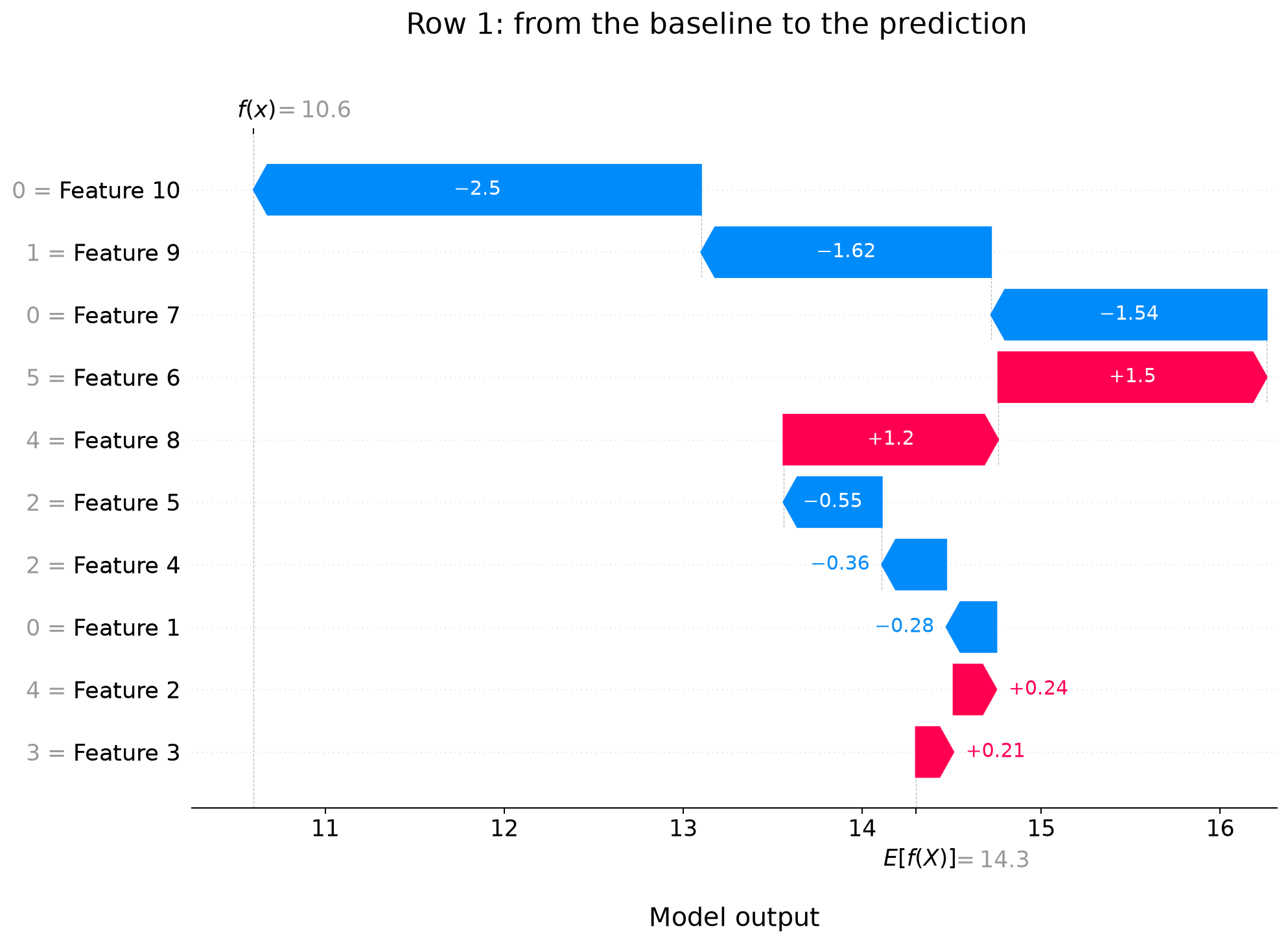
For row 1, the baseline is \(14.30\) and the prediction is \(10.60\). The fitted contributions sum to \(-3.70\), giving \(14.30 + (-3.70) = 10.60\).
The waterfall plot shows how those contributions add up. Read from the baseline at the bottom towards the prediction at the top: red bars increase the prediction and blue bars decrease it until we reach the prediction for row \(1\). The features are ordered by the size of their absolute contributions; the labels also show their values in this row.
The original SHAP paper derives this kernel, and the KernelExplainer documentation describes how to use background data with an existing model.
Final Thoughts
This was a lot of maths, and you made it! Congratulations! I hope that you can now understand how SHAP values are computed. They explain the contribution of each feature value to a model prediction. The calculations on this page are purely illustrative. In practice, you would use a library like shap to compute them for the model you trained. Still, it is good discipline to look under the hood once in a while.
What predictions do you now want to explain?