Book Notes: Maximum Likelihood hides everywhere
As a budding Data Scientist, I long thought that I could avoid the concept of Maximum Likelihood altogether. I kept telling myself that I was just using easy-to-grasp distance metrics like Mean Squared Error (MSE) for regression and any kind of confusion matrix derivatives for classification.
As it turns out, Maximum Likelihood hides everywhere, and this is what I will try to show with this article. It will describe the point highlighted by Simon Prince in his majestic Understanding Deep Learning book: if you are scoring a model with the Mean Squared Error, you are using Maximum Likelihood and making several assumptions you are not aware of. Let’s get into it!
Note: For more insightful bits of Machine Learning theory, I would strongly recommend reading Understanding Deep Learning as an ebook or buying a hard copy.
Agreeing on Machine Learning basics
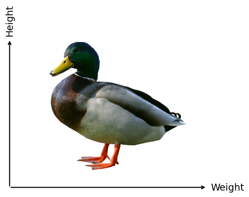
The objective of a Machine Learning model is to learn a function \(f(x,\phi)\), which will output conditional probabilities of the target variable \(y\), given a feature vector \(x\). This conditional probability distribution is noted \(P(y \mid x)\), or \(P\bigl(y \mid f(x,\phi)\bigr)\).
As an example, you may want to predict the height of a duck based (\(y\)) on its weight (\(x\)). Your model would output, for every value of the weight \(x\) a probability distribution of different height values. If you did a good modelling job, the heigher the weight of the duck \(x\) the taller the duck (\(y\)).
Code used to generate the plot
import matplotlib.pyplot as plt
import matplotlib.image as mpimg

img = mpimg.imread('duck.png')

fig = plt.figure(figsize=(8, 6))

ax_arrows = fig.add_axes([0.1, 0.1, 0.5, 0.5])

ax_arrows.set_xticks([])
ax_arrows.set_yticks([])
for spine in ax_arrows.spines.values():
    spine.set_visible(False)

ax_arrows.annotate(
    '',
    xy=(1, 0),
    xytext=(0, 0),
    xycoords='data',
    arrowprops=dict(arrowstyle='->', color='black', lw=1.5)
)

ax_arrows.annotate(
    '',
    xy=(0, 1),
    xytext=(0, 0),
    xycoords='data',
    arrowprops=dict(arrowstyle='->', color='black', lw=1.5)
)

ax_arrows.text(
    1.02, 0, 'Weight',
    fontsize=14,
    ha='left', va='center',
    transform=ax_arrows.transData
)
ax_arrows.text(
    0, 1.02, 'Height',
    fontsize=14,
    ha='center', va='bottom',
    rotation=90,
    transform=ax_arrows.transData
)

ax_duck = fig.add_axes([0.2, 0.15, 0.35, 0.45])
ax_duck.imshow(img)

ax_duck.axis('off')

plt.show()
This is a regression problem. The classification equivalent would be to classify animals, assigning probabilities to labels like “duck” or “swan” (\(y\)) based on their height and weight (feature vector \(\boldsymbol{x}\)).
What is Maximum Likelihood?
We want to find the model that is the most “likely” based on our data. This model replicates the system we are trying to model.
Let’s say we are predicting the clinical risk of a patient admitted into an A&E service based on their medical history and current symptoms. The most likely model is the model that most accurately predicts the patient outcome based on their features, over the training data.
We would like, for each patient outcome (in our historical data), to find the model parameters \(\hat{\phi}\) that maximise the following quantity (big formula warning):
\[ \prod_{i} p\bigl(y_i \mid f(x_i,\phi)\bigr) \]
Some important points to note:
- \(i\) is a patient
- \(y_i\) is the patient outcome (fatality, discharge, stay longer than 2 days…)
- \(x_i\) is the vector representing the patient’s medical history and current symptoms
- \(f(x_i,\phi)\) is the model output based on a given patient’s features, and a given set of model parameters
Observations do need to be independent from one another, expand this to understand why
A critical assumption of this to hold is the assumption that all rows are independent and identically distributed (i.i.d), a common assumption in Machine Learning practice. The idea is that the outcome of a patient (one row) should not be correlated with another patient’s outcome (any other row).
If there is a correlation, then the following equality does not hold:
\[ P(y_1, y_2, \ldots, y_n \mid x_1, x_2, \ldots, x_n) \;=\; \prod_{i} p\bigl(y_i \mid f(x_i,\phi)\bigr) \]
Remember that the intersection of two events is \[ P(A \cap B) = P(A)\times P(B \mid A) \]
When \(A\) and \(B\) are independent, \(P(B \mid A) = P(B)\), which allows us to compute the intersection with a simple product: \[ P(A \cap B) = P(A)\times P(B) \]
Finding the Maximum Likelihood
Products are notoriously difficult to optimise. To do so, we can leverage two useful mathematical tricks of optimisation (maths warning):
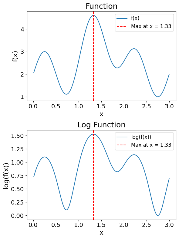
- The maximum of a function over the range \((0,\infty)\) will be reached at the maximum of the \(\log\) of that function.
- The logarithm of a product is equivalent to the sum of the logarithm of its terms.
Understanding both of these using English, \(log(x)\) is a monotonically increasing function over the range \((0,\infty)\). This means that the \(\log\) of a function \(f(x)\), noted \(\log(f(x))\), will reach its maximum at the same point as \(f(x)\).
Code used to generate the plot
import numpy as np
import matplotlib.pyplot as plt

x = np.linspace(0.01, 3, 400)
y = np.sin(2*np.pi*x) + 2.0
logy = np.log(y)

fig, axs = plt.subplots(2, 1, figsize=(6, 8))
axs[0].plot(x, y)
axs[0].set_title('Function', fontsize=18)
axs[0].tick_params(axis='both', labelsize=14)
axs[0].set_xlabel('x', fontsize=16)
axs[0].set_ylabel('f(x)', fontsize=16)

axs[1].plot(x, logy)
axs[1].set_title('Log of Function', fontsize=18)
axs[1].tick_params(axis='both', labelsize=14)
axs[1].set_xlabel('x', fontsize=16)
axs[1].set_ylabel('log(f(x))', fontsize=16)

plt.tight_layout()
plt.show()
One of the useful properties of logarithms is that the log of a product is equal to the sum of the logs of its terms: \(\log(a \cdot b) = \log(a) + \log(b)\).
Why is this the case?
Using logarithms base 2 for simplicity. e.g., \(\log(a) = 2^a\) and \(\log(8) = 3\)
\(\begin{align} \text{Let } x &= \log(a \cdot b) \\ 2^x &= a \cdot b, \text{ exponentiating both sides, by definition: } 2^{\log(a \cdot b)} = a \cdot b \\ 2^x &= 2^{\log(a)} \cdot 2^{\log(b)}, \text{ by definition: } 2^{\log(a)} = a \text{ the same for } b \\ 2^x &= 2^{\log(a) + \log(b)}, \text{ by the exponent addition rule: } 2^a \cdot 2^b = 2^{a+b} \\ x &= \log(a) + \log(b), \text{ taking the logarithm of both sides} \\ \log(a \cdot b) &= \log(a) + \log(b), \text{ substituting } x = \log(a \cdot b) \end{align}\)
With this proven, let’s get back to our Maximum Likelihood.
Going back to our problem, we need to find the set of parameters \(\hat{\phi}\) maximising the likelihood function:
\[ \hat{\phi} = \arg\max_{\phi} \prod_{i} p\bigl(y_i \mid f(x_i,\phi)\bigr) \]
This parameter set will also maximise the following function:
\[ \log \Bigl(\prod_{i} p\bigl(y_i \mid f(x_i,\phi)\bigr)\Bigr) \;=\; \sum_{i} \log p\bigl(y_i \mid f(x_i,\phi)\bigr). \]
But what about negative log-likelihood? Why is this term also everywhere if we try to maximise log-likelihood?
By convention, when fitting models, we aim to minimise loss. For this reason, instead of maximising log-likelihood, we minimise negative log-likelihood:
\[ \hat{\phi} = \arg\min_{\phi} - \sum_{i} \log p\bigl(y_i \mid f(x_i,\phi)\bigr). \]
This type of manipulations is very common in optimisation.
Mean Squared Error and Maximum Likelihood
Let’s start with a basic regression problem in which we model the height of a duck (\(y\)) based on its weight (\(x\)), using a model \(f(x, \phi)\), with parameters \(\phi\).
We model the height of a duck as a function of its weight, with some random noise: \[ y = f(x,\phi) + e \]
with \(e\) some Gaussian noise with the following distribution: \[ e \sim N(0,\sigma^2). \]
Hence, the height of ducks follows the distribution \[ y \mid x \sim N\bigl(f(x,\phi),\sigma^2\bigr). \]
Until now, we have not said much. The model is simply outputting a distribution over each height value based on different weight values.
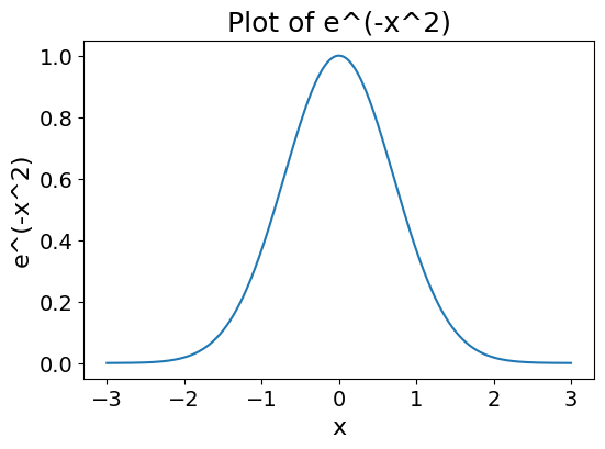
The probability density function of the normal distribution can be scary. The way I try to think about it is that it is approximately \(\mathrm{e}^{-x^2}\), scaled so that it integrates to 1.
Expand this if you don’t believe me
import numpy as np
import matplotlib.pyplot as plt

x = np.linspace(-3, 3, 400)
y = np.exp(-x**2)

fig, ax = plt.subplots(figsize=(6,4))
ax.plot(x, y)
ax.set_title('Plot of e^(-x^2)', fontsize=18)
ax.set_xlabel('x', fontsize=16)
ax.set_ylabel('e^(-x^2)', fontsize=16)
ax.tick_params(axis='both', labelsize=14)
plt.show()
The probability density function of the normal distribution is as follows:
\[\begin{align*} p(y \mid \mu, \sigma^2) &= \frac{1}{\sqrt{2 \pi \sigma^2}} \exp\Bigl(-\frac{(y-\mu)^2}{2\sigma^2}\Bigr). \tag{1} \end{align*}\] Let’s say our model uses parameters \(\phi\) and features \(x\) to predict the mean height \(\mu\). We get:
\[\begin{align*} \hat{\mu} &= f(x,\phi) \end{align*}\]
Since our model \(f(x,\phi)\) predicts the mean \(\mu\), we can substitute this into equation (1):
\[\begin{align*} p\bigl(y \mid f(x,\phi), \sigma^2\bigr) &= \frac{1}{\sqrt{2\pi\sigma^2}} \exp\Bigl(-\frac{\bigl(y - f(x,\phi)\bigr)^2}{2\sigma^2}\Bigr). \tag{3} \end{align*}\]
For our entire dataset \(\{(x_i,y_i)\}_{i=1}^n\), the likelihood becomes: \[\begin{align*} \prod_{i=1}^n p\bigl(y_i \mid f(x_i,\phi), \sigma^2\bigr) &= \prod_{i=1}^n \left[ \frac{1}{\sqrt{2\pi\sigma^2}} \exp\Bigl(-\frac{(y_i - f(x_i,\phi))^2}{2\sigma^2}\Bigr) \right]. \tag{4} \end{align*}\] Taking the negative log-likelihood (which we want to minimise):
\[\begin{align*} &-\log\left(\prod_{i=1}^n p\bigl(y_i \mid f(x_i,\phi), \sigma^2\bigr)\right) \\ &= -\sum_{i=1}^n \log\left( \frac{1}{\sqrt{2\pi\sigma^2}} \exp\Bigl(-\frac{(y_i - f(x_i,\phi))^2}{2\sigma^2}\Bigr) \right). \tag{5} \end{align*}\]
Using the properties of logarithms to split the terms of the product:
\[\begin{align*} &= -\sum_{i=1}^n \left[ \log\Bigl(\frac{1}{\sqrt{2\pi\sigma^2}}\Bigr) + \log\Bigl(\exp\bigl(-\frac{(y_i - f(x_i,\phi))^2}{2\sigma^2}\bigr)\Bigr) \right]. \tag{6} \end{align*}\]
Simplifying by splitting the sum into two sums:
\[\begin{align*} &= -\sum_{i=1}^n \left[ -\log\bigl(\sqrt{2\pi\sigma^2}\bigr) - \frac{(y_i - f(x_i,\phi))^2}{2\sigma^2} \right] \\ &= \sum_{i=1}^n \log\bigl(\sqrt{2\pi\sigma^2}\bigr) + \sum_{i=1}^n \frac{(y_i - f(x_i,\phi))^2}{2\sigma^2}. \tag{7} \end{align*}\] The first term \(\sum_{i=1}^n \log\bigl(\sqrt{2\pi\sigma^2}\bigr)\) is constant with respect to \(\phi\). Therefore, minimising the negative log-likelihood with respect to \(\phi\) is equivalent to minimising:
\[\begin{align*} \sum_{i=1}^n \frac{(y_i - f(x_i,\phi))^2}{2\sigma^2}. \tag{8} \end{align*}\]
Since \(\sigma^2\) is also constant with respect to \(\phi\), we can further simplify to:
\[\begin{align*} \sum_{i=1}^n (y_i - f(x_i,\phi))^2 \tag{9} \end{align*}\]
which is the Mean Squared Error (MSE).
The key assumption is that the noise around \(f(x_i,\phi)\) is normally distributed with mean 0 and constant variance \(\sigma^2\), making MSE the natural choice for the loss when these conditions hold.
What happens when the variance \(\sigma^2\) is not constant?
Constant variance of error or Gaussian “noise” is one of the assumptions you make when using the Mean Squared Error as an error metric. This is commonly used with Ordinary Least Squared regression.
Traumatised students may remember the scary homoskedasticity term. This is the assumption of constant variance. When variance is not constant, the problem becomes heteroskedastic, which require other modelling choices. In such modelling, minimising the Mean Squared Error does not minimise negative log-likelihood.
I could not believe my eyes the first time I saw this. By using the MSE, you are actually assuming Gaussian noise around your model and finding the model parameters that minimise negative log-likelihood. A good reminder to check your assumptions.
Final Thoughts
This was a bit of maths, hopefully worth it. Some key points:
- Maximum Likelihood is everywhere in Machine Learning.
- Maximising a function over the range \((0,\infty)\) is equivalent to maximising the log of this function.
- Maximising a product is tough, but the log of a product is the sum of its terms.
This is one of the many examples brilliantly explained by Simon Prince in Understanding Deep Learning. If you liked it, I would recommend reading the ebook and/or buying a hard copy.