Understanding Gini Impurity in Decision Tree Learning

While preparing for an introductory course on Machine Learning, I realised that I could not explain what the Gini Impurity criterion was. I understood that it measured how well groups of observations were separated, but the way it was actually computed still eluded me.

After some Wikipedia research, I discovered that there was a simple way to understand this criterion, which turned out to be an elegant way to measure how heterogeneous a group is. This blog will develop this intuition.

If you are not a Machine Learning practitioner, do not leave yet. Read through the example below first; you may still be interested.

Let’s say you have two playlists and want to know which playlist is the most diverse. These two playlists are called Playlist A and Playlist B (very creative, I know). They are composed of two genres, Pop and Rock. If you would like to see more genres in the playlist, read on.

Playlist	Pop	Rock
Playlist A	90	10
Playlist B	60	40

The table above shows each playlist’s number of songs from each of the two genres.

The question is, what playlist is most diverse?

Your immediate answer will probably be: “Playlist B, of course, but where are you going with this example?”.

I agree with you, it is Playlist B. Now, how could you measure the diversity of these two playlists with a single number? This is the problem Gini Impurity tries to tackle.

Motivation

In modern Machine Learning practice, a model named Decision Tree is absolutely everywhere. This model uses Gini Impurity to split data into homogeneous groups. You do not need to know this to read this article, as it will focus on Gini Impurity and the diversity of our two playlists.

If you are a Machine Learning practitioner, simply replace the playlists with two groups in a classification problem.

Intuition

Gini Impurity is a single number describing how impure or heterogeneous a group is. This number should be high when the group is mixed and low when the group is pure. Using our playlist example, it should be high when the playlist is diverse and low when the playlist mainly contains songs of one genre.

How would you summarise this degree of impurity using a single number?

Gini Impurity does so in a very elegant way, by computing the probability of randomly picking (with replacement) two elements of a different class. If that probability is high, it means that group is impure; if it is low, the group is considered pure.

Starting with our example, if I play Playlist A on shuffle (with songs in a random order), it is very likely that any two consecutive songs will be of the same “Pop” genre. However, in Playlist B, this is less clear-cut. In shuffle mode, we would expect two consecutive songs to have a different genre more often.

It is that probability of picking two songs of a different genre that the Gini Impurity measures.

As a quick note, the playlist example I just gave is not fully correct. When you set a playlist to shuffle mode, the next song is actually not a fully random choice. If it was, the same song could be played twice. To be in line with the Gini Impurity calculation, the next song selection should be fully random, including the possibility of picking the same song twice. The difference between the two, with and without replacement, is very small for large playlists anyway.

Diving into the Maths

Now let’s get into the maths. We want to compute the probability of picking two songs of a different genre. We do so with replacement, allowing for the possibility to pick the same song twice. In other words, we randomly select a song from the full playlist in both cases.

Playlist	Pop	Rock
Playlist A	90	10
Playlist B	60	40

We will start by defining classes, here the different music genres. We will note “Pop” as 1 and “Rock” as 2.

We note \(p_1\) and \(p_2\) as the frequency of “Pop” and “Rock” songs within a playlist. It is noted \(p_{i}\) as it is also the probability of randomly picking a song of each genre.

Frequencies and Probabilities

The probability is the measure of the likelihood of an event happening. It is also sometimes referred to as a degree of belief. It is a theoretical concept that quantifies uncertainty; i.e., that puts a number on something we do not know. Probabilities are expressed as a number between \(0\) and \(1\); \(0\) being the probability of an uncertain event, and \(1\) the probability of a certain event.

Example: The probability of getting “head” when flipping a fair coin is \(\frac{1}{2}\).

The frequency refers to the number of times an event occurs within a given set of trials. It is an empirical measure based on actual data. It is calculated as follows:

\[ \text{Frequency} = \frac{\text{Number of times an event occurs}}{\text{Total Number of trials}} \]

Example: If you flip a fair coin three times and get “head” twice, the frequency of getting “head” is \(\frac{2}{3}\).

Note that these two statements are not contradictory. The law of large numbers ties these two concepts together. It states that over a large number of trials, the frequency of an event will converge towards its probability.

Example: The following chart shows the frequency of getting “head” when flipping a fair coin. As the number of trials increases, the frequency converges towards the probability of \(\frac{1}{2}\).

The frequency converges towards the theoretical probability as the number of trials increases.

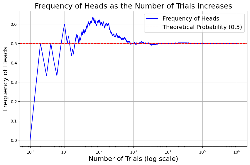
Code used to generate the plot

import numpy as np
import matplotlib.pyplot as plt

max_trials = 10**6
coin_flips = np.random.randint(0, 2, size=max_trials)
cumulative_heads = np.cumsum(coin_flips)
trial_numbers = np.arange(1, max_trials + 1)
relative_frequency = cumulative_heads / trial_numbers

plt.figure(figsize=(10, 6))
plt.plot(trial_numbers, relative_frequency, label="Relative Frequency of Heads", color="blue")
plt.axhline(y=0.5, color="red", linestyle="--", label="Theoretical Probability (0.5)")
plt.xscale("log")
plt.xlabel("Number of Trials (log scale)", fontsize=16)
plt.ylabel("Relative Frequency", fontsize=16)
plt.title("Law of Large Numbers Simulation with a Fair Coin", fontsize=18)
plt.legend(fontsize=14)
plt.grid(True)
plt.show()

Back to our example, the frequency of Pop songs in Playlist A is:

\[ p_1 = \frac{90}{90 + 10} = 0.9 \]

As a consequence, if I were to randomly select a song in Playlist A, I would have a probability of 0.9 to pick a Pop song.

The first sentence of the last paragraph is an empirical observation. The second is a theoretical argument.

As an example, for Playlist A:

\[ p_1 = \frac{90}{90 + 10} = 0.9, \quad p_2 = \frac{10}{90 + 10} = 0.1 \]

If the first song we pick is a Pop song, what is the probability of picking a Rock song next? It is \(p_2\) or 0.1 as both events are independent. In other words, the first song choice is a random choice that does not influence the second choice.

As the two events are independent, the probability of picking a Pop song and then a Rock song can be computed as follows:

\[ p_1 \cdot p_2 = 0.9 \cdot 0.1 = 0.09 \]

Preparing for the more general case of more than two classes, we are actually interested in the probability of picking a Pop song, followed by picking “not a Pop” song. This can be computed as:

\[ p_1 \cdot (1 - p_1) = 0.9 \cdot (1 - 0.9) = 0.9 \cdot 0.1 = 0.09 \]

In the binary case, this does not make any difference but will be useful if we have more than two classes.

Our job is not done yet. To get the Gini Impurity, we need the probability of any two randomly selected songs having a different genre. We have just covered the case: “Pop then not Pop”. We need to do this for all other classes.

Applying this to Playlist A for the Rock genre (class 2), we can compute the probability of picking “Rock then not Rock” as follows:

\[ p_2 \cdot (1 - p_2) = 0.1 \cdot (1 - 0.1) = 0.1 \cdot 0.9 = 0.09 \]

You can see that this is the same result as the “Pop then not Pop”. This is by symmetry as we just have two classes. It will get a bit more exciting with more classes.

To get the Gini Impurity, we will sum this probability of mismatch for all classes. For Playlist A, we get:

\[ \text{Gini Impurity} = p(\text{Pop then not Pop}) + p(\text{Rock then not Rock}) = 0.09 + 0.09 = 0.18 \]

This number is close to 0, which makes sense as Playlist A is relatively pure; in other words, not very diverse.

Playlist	Pop	Rock
Playlist A	90	10
Playlist B	60	40

To test your understanding, calculate the Gini Impurity of Playlist B. Does this confirm your intuition?

Answer

For Playlist B:

\[ p_1 = \frac{60}{60 + 40} = 0.6, \quad p_2 = \frac{40}{60 + 40} = 0.4 \]

\[ \text{Gini Impurity} = p_1 \cdot (1 - p_1) + p_2 \cdot (1 - p_2) = 0.6 \cdot 0.4 + 0.4 \cdot 0.6 = 0.24 + 0.24 = 0.48 \]

This confirms that Playlist B is more diverse than Playlist A.

Moving to More Classes (and Big Formula Warning)

If your goal was just to understand the intuition behind Gini Impurity, congrats, you’ve done it. You can skip directly to the conclusion. This section will introduce the general Gini Impurity formula, hence the big formula warning in the title.

As defined above, Gini Impurity measures the probability of picking two items (with replacement) of a different class. We define \(J\) as the number of classes, \(i \in \{1, 2, \dots, J\}\). \(p_i\) is the frequency of any given class.

\[ \text{Gini Impurity} = \sum_{i=1}^J p_i \cdot (1 - p_i) \]

This formula may be scary because of the summation operator, but it simply means add up \(p_i \cdot (1 - p_i)\) for all \(i\) classes. Exactly what we did with the playlist examples. Let’s apply this formula to the previous example with an additional genre.

Example with Three Classes

Adding Folk to the playlists, the updated table is as follows:

Playlist	Pop	Rock	Folk
Playlist A	70	20	10
Playlist B	50	30	20

Can you calculate the Gini Impurity for Playlist A and Playlist B using the general formula?

Hint: Compute \(p_i\) for each class and then substitute into the formula.

Solution

For Playlist A: \[ p_1 = \frac{70}{70 + 20 + 10} = 0.7, \quad p_2 = \frac{20}{70 + 20 + 10} = 0.2, \quad p_3 = \frac{10}{70 + 20 + 10} = 0.1 \]

\[ \text{Gini Impurity} = p_1 \cdot (1 - p_1) + p_2 \cdot (1 - p_2) + p_3 \cdot (1 - p_3) \]

\[ \text{Gini Impurity} = 0.7 \cdot 0.3 + 0.2 \cdot 0.8 + 0.1 \cdot 0.9 = 0.21 + 0.16 + 0.09 = 0.46 \]

For Playlist B:

\[ p_1 = \frac{50}{50 + 30 + 20} = 0.5, \quad p_2 = \frac{30}{50 + 30 + 20} = 0.3, \quad p_3 = \frac{20}{50 + 30 + 20} = 0.2 \]

\[ \text{Gini Impurity} = p_1 \cdot (1 - p_1) + p_2 \cdot (1 - p_2) + p_3 \cdot (1 - p_3) \]

\[ \text{Gini Impurity} = 0.5 \cdot 0.5 + 0.3 \cdot 0.7 + 0.2 \cdot 0.8 = 0.25 + 0.21 + 0.16 = 0.62 \]

This confirms that Playlist B is more diverse than Playlist A.

Final Thoughts

Gini Impurity is a very elegant measure of diversity within a group. It does so by measuring the probability of randomly selecting two elements of a different class. It has applications in many fields such as economics and Machine Learning.

It is also an example of reducing a qualitative observation (“diversity”) into a single, easy-to-compute number. This is one of the key concepts of optimisation. To maximise or minimise an objective, you have to quantify it first.

Is there a way you could apply Gini Impurity to your current problems? Is there a qualitative observation you could reduce to a single number? Some food for thought.