Double ML: Bridging the Gap Between Machine Learning and Causal Inference

Author

Eliott Kalfon

Published

February 22, 2025

Subscribe to my newsletter to hear about my latest posts. No spam, I promise.

What will the weather be tomorrow? If I lower the price of my beer by 10%, by how much will my sales increase?

These two questions may look the same. In both cases, we are concerned with a prediction; we want to know what will happen tomorrow.

This is all too human. We have always wanted to know the unknowable, to predict the future, to put order in chaos.

Supervised Machine Learning

Machine Learning (ML) methods are one of the best tools we have to predict the future using historical data. ML models answer the question: what will happen tomorrow, assuming that the process generating the historical data is the same as the process generating tomorrow’s data?

This may sound convoluted, though the idea is simple. In Machine Learning, we assume that there is a process, hidden from us, that generates the facts/data we observe. As an example, we assume that the process that has generated the last 10 years of weather data will also generate tomorrow’s weather data.

When we train Machine Learning models, we try to learn this data generation process and use it to make predictions. These models learn that a cloudy night will probably lead to rain the next day, or that an east-moving cloud over Frankfurt may arrive in Berlin in a day or two. These models map past observations to future events:

Cloudy night $⟹$ Rainy day
East moving cloud over Frankfurt $⟹$ Cloud over Berlin soon

It will leverage correlations between input and output data.

This approach works very well when our task is simply to predict, nothing else. When you just want to know what the weather will be tomorrow.

The second question has an additional dimension: If I lower the price of my beer by 10%, by how much will my sales increase?

There, we want to know what will happen if we make an action. We want to know the additional beers we will sell if we lowered the price by 10%.

We could be tempted to use the same reasoning as above and train an ML model to learn the relationship between sales and price/discount. We would then predict the sales using different prices. Job done, feels great being a Data Scientist…

Unfortunately, this rarely works, for a few different reasons.

First, Machine Learning assumes that there is a single data-generating process. There is a hidden function that generates beer sales based on price and other features. We try to learn this function by training a Machine Learning model. If, when we predict, we change our usual way to price—for example, pricing much lower than usual—our model will have no way to know the impact this will have on our sales. This will be outside of the model’s training data.

Second, correlation and causation do not always go well together. Let’s say, for instance, that your model predicts lower sales when you lower the price of the beer. How can this be possible? This makes no sense at all… And yet, ML models are not in the business of making sense; they are in the prediction business. Correlation is all that matters.

Let’s try to understand how such a phenomenon could come about. Let’s say that you generally lower prices when you struggle to sell a particular type of beer. Then, in your historical data, lower prices are correlated with low demand for the beer. A model could then learn that when prices are lower, demand is low too. Even though this seems counterintuitive to a human, this will actually help a model make better sales predictions.

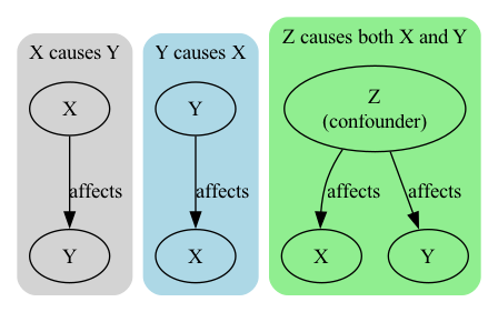
This shows that three different causal relationships between two variables $X$ and $Y$ (here price and sales) can show up as correlation in your data:

$X$ causes $Y$
$Y$ causes $X$
$Z$ (a third variable, like an exceptional event, e.g., a football world cup) causes both $X$ and $Y$

Machine Learning models will not care the least and use values of $X$ to predict $Y$ anyway. This may help if you are just interested in sales predictions, but it will not help you in setting your prices correctly.

Causal Inference to the Rescue

It is important to distinguish traditional supervised Machine Learning and Causal Inference methods.

Whereas Machine Learning models predict $Y$ given $X$ , Causal Inference methods predict $Y$ given an action over $X$ , also noted $do (X)$ .

There are many ways to do Causal Inference; it is a fascinating topic. My favourite books on this are Statistical Rethinking by McElreath and The Book of Why by Pearl.

Today we will focus on Double Machine Learning (DML), an elegant approach developed by Chernozhukov et al. ¹.

Let’s describe it with our simple beer sales example, in which:

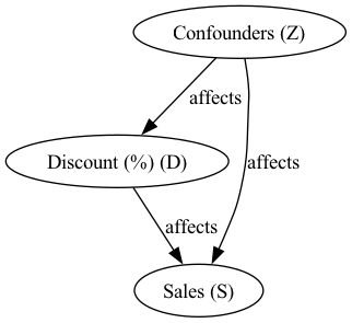
Beer sales ( $S$ ) are influenced by both discount percentage ( $D$ ) and a set of confounders ( $Z$ ), including previous sales, calendar, seasonality, etc. In other words, these confounders are everything that affects sales that are not discount percentage.
In our data, higher discounts (lower prices) are also correlated with lower demand, as they are used to increase sales in low-demand periods.

Example shown in a Directed Acyclic Graph (DAG)

We can generate a synthetic dataset with these properties:

Expand to show the distributions used to generate the synthetic dataset. If formulas are not your thing, read on

Confounders ( $Z$ ): We assume $Z \sim N (50, 10^{2})$ , representing baseline levels (e.g., underlying demand or seasonality) that drive both the discount strategy and sales.
Discount ( $D$ ): $D = 40 - 0.3 \cdot Z + ϵ_{D}, ϵ_{D} \sim N (0, 2^{2})$ This means that when $Z$ is low (i.e., low demand expected), the discount is set higher.
Sales ( $S$ ): $S = 100 + 5 \cdot D + 2 \cdot Z + ϵ_{S}, ϵ_{S} \sim N (0, 5^{2})$ Note that both the discount (which tends to increase sales) and the underlying demand ( $Z$ ) contribute positively to sales. The relationship between $D$ and $S$ of 5 (i.e., 1 more unit of discount leads to 5 more additional units of sales) is what we will want to recover using Double ML.

Pairplot of the dataset, note that discounts are correlated with lower sales, a counter intuitive result

Code used to generate the dataset and plot


import numpy as np
import pandas as pd
import matplotlib.pyplot as plt
import seaborn as sns

np.random.seed(42)
n = 1000

Z = np.random.normal(loc=50, scale=10, size=n)  # e.g., baseline level of demand

# Generate Discount (D) - notice negative correlation with confounder
D = 40 - 0.5 * Z + np.random.normal(loc=0, scale=2, size=n)  # discount percentage

# Generate Sales (S)
# Sales are positively influenced by both the discount (D) and the baseline demand (Z).
S = 100 + 5 * D + 4 * Z + np.random.normal(loc=0, scale=5, size=n)

# Create a DataFrame
data = pd.DataFrame({'Z': Z, 'D': D, 'S': S})

# Plot
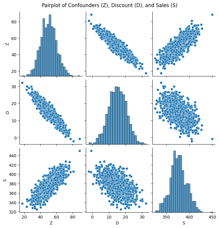
sns.pairplot(data)
plt.suptitle('Pairplot of Confounders (Z), Discount (D), and Sales (S)', y=1.02)
plt.show()

Note the negative correlation between Sales (S) and Discount (D). This is due to the fact that Discounts are increased in low demand periods, when the beer doesn’t sell.

Double Machine Learning Implementation

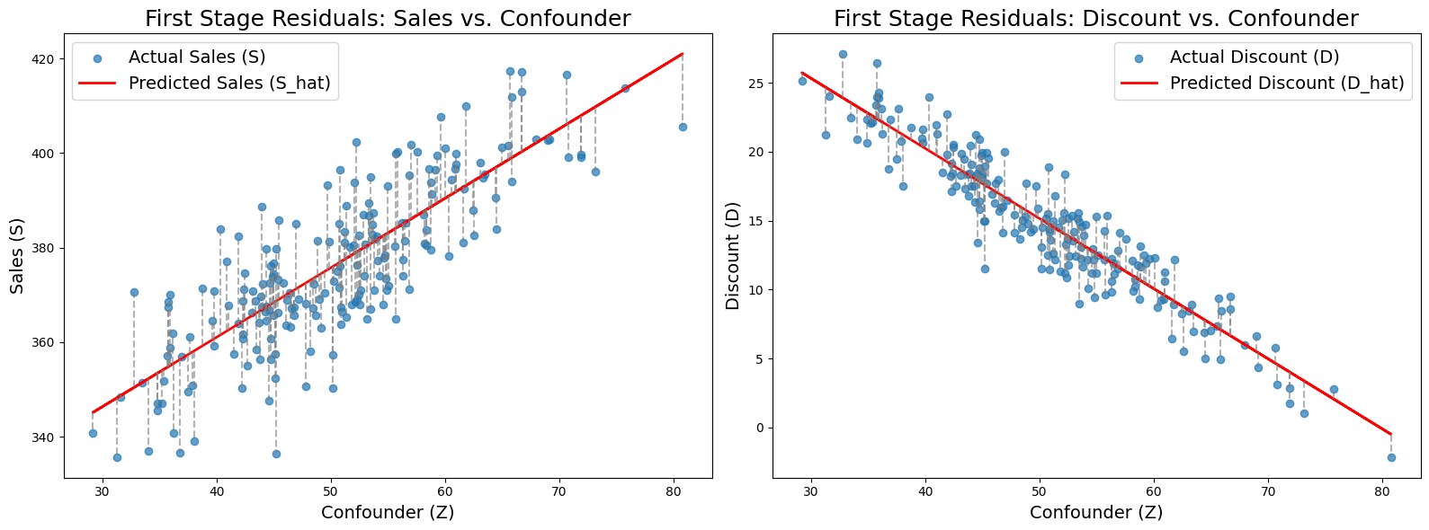
Now that the stage is set, let’s get into the Machine Learning part of it. We first train two Machine Learning models:

One model uses the confounders ( $Z$ ) to predict the discount ( $D$ )
Another model uses the confounders ( $Z$ ) to predict sales ( $S$ )

We then sample the errors of both models. These errors capture:

All of the discount information that cannot be predicted from confounders $Z$
All of the sales information that cannot be predicted from confounders $Z$

Residuals (prediction errors) of both first stage models

Code used to generate the plots


import numpy as np
import matplotlib.pyplot as plt

sorted_data = data.sort_values(by='Z').sample(n=200, random_state=42).reset_index(drop=True)
Z_sorted = sorted_data['Z'].values

S_actual = sorted_data['S'].values
S_fit    = sorted_data['S_hat'].values  # predicted S from reg_S

D_actual = sorted_data['D'].values
D_fit    = sorted_data['D_hat'].values  # predicted D from reg_D

fig, axes = plt.subplots(1, 2, figsize=(16, 6))

# --- Left Plot: S (Sales) vs. Z ---
axes[0].scatter(Z_sorted, S_actual, alpha=0.7, label='Actual Sales (S)')
# Plot the fitted regression line
axes[0].plot(Z_sorted, S_fit, color='red', linewidth=2, label='Predicted Sales (S_hat)')
# Draw vertical lines connecting actual S to the fitted value S_hat
axes[0].vlines(Z_sorted, S_fit, S_actual, color='gray', linestyle='--', alpha=0.6)
axes[0].set_xlabel('Confounder (Z)')
axes[0].set_ylabel('Sales (S)')
axes[0].set_title('First Stage Residuals: Sales vs. Confounder')
axes[0].legend()

# --- Right Plot: D (Discount) vs. Z ---
axes[1].scatter(Z_sorted, D_actual, alpha=0.7, label='Actual Discount (D)')
# Plot the fitted regression line
axes[1].plot(Z_sorted, D_fit, color='red', linewidth=2, label='Predicted Discount (D_hat)')
# Draw vertical lines connecting actual D to the fitted value D_hat
axes[1].vlines(Z_sorted, D_fit, D_actual, color='gray', linestyle='--', alpha=0.6)
axes[1].set_xlabel('Confounder (Z)')
axes[1].set_ylabel('Discount (D)')
axes[1].set_title('First Stage Residuals: Discount vs. Confounder')
axes[1].legend()

plt.tight_layout()
plt.show()

We then use the errors of the first model (predicting discount) to predict the errors of the second model (predicting sales). This should give us an unbiased estimation of the effect of discounts on sales.

Plotting the relationship of the residuals of the two models shows a positive correlation between discount and sales after controlloing for confounders. The slope of 5 is the effect that had been built into this synthetic dataset.

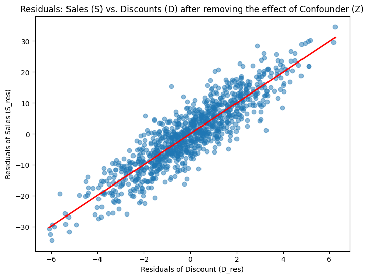
Predicting sales residuals using discount residuals

Code used to implement Double ML and plot residuals


from sklearn.linear_model import LinearRegression
import statsmodels.api as sm

reg_S = LinearRegression().fit(data[['Z']], data['S'])
reg_D = LinearRegression().fit(data[['Z']], data['D'])

data['S_hat'] = reg_S.predict(data[['Z']])
data['D_hat'] = reg_D.predict(data[['Z']])

data['S_res'] = data['S'] - data['S_hat']
data['D_res'] = data['D'] - data['D_hat']

reg_double_ml = LinearRegression().fit(data[['D_res']], data['S_res'])
double_ml_coef = reg_double_ml.coef_[0]
double_ml_intercept = reg_double_ml.intercept_

print("\nDouble ML Regression Results (scikit-learn):")
print("Estimated coefficient on D_res (promotional effect):", double_ml_coef)
print("Estimated intercept:", double_ml_intercept)

X_sm = sm.add_constant(data['D_res'])
model = sm.OLS(data['S_res'], X_sm).fit()
print("\nDouble ML Regression Summary (statsmodels):")
print(model.summary())

plt.figure(figsize=(8, 6))
plt.scatter(data['D_res'], data['S_res'], alpha=0.5)
plt.xlabel('Residuals of Discount (D_res)')
plt.ylabel('Residuals of Sales (S_res)')
plt.title('Residuals: Sales (S) vs. Discounts (D) after removing the effect of Confounder (Z)')

x_vals = np.linspace(data['D_res'].min(), data['D_res'].max(), 100)
y_vals = double_ml_intercept + double_ml_coef * x_vals
plt.plot(x_vals, y_vals, color='red', linewidth=2)
plt.show()

Congratulations for making it this far, this was exactly what we were looking for. Through Double Machine Learning, we were able to find the causal impact of discounts on sales despite the presence of a confounder. This model could now be used in practice to estimate the impact of discounts on beer sales.

The following example is very simplified. One of the many advantages of Double Machine Learning is that this approach supports any kind of modelling approach. You could use Deep Learning models to predict sales and discounts from confounders $Z$ .

Final Thoughts

Double ML is a very flexible approach to causal inference, a good start for Machine Learning practitioners. Whenever you are trying to move from prediction to action, this is an important framework to consider. Can you already think of an application in your day-to-day work?

Footnotes

Chernozhukov, V., Chetverikov, D., Demirer, M., Duflo, E., Hansen, C., Newey, W., & Robins, J. (2018). Double/debiased machine learning for treatment and structural parameters.↩︎

Supervised Machine Learning

Causal Inference to the Rescue

Double Machine Learning Implementation

Final Thoughts

Footnotes

Like what you read? Subscribe to my newsletter to hear about my latest posts!